Functions with R

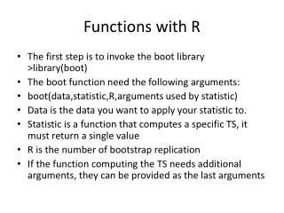
1. Functions with R • The first step is to invoke the boot library>library(boot) • The boot function need the following arguments: • boot(data,statistic,R,arguments used by statistic) • Data is the data you want to apply your statistic to. • Statistic is a function that computes a specific TS, it must return a single value • R is the number of bootstrap replication • If the function computing the TS needs additional arguments, they can be provided as the last arguments

2. Creating the appropriate function to pass to the statistic argument • The function boot uses the function provided in the statistic argument to sample “something” with replacement. In this course, we will only see the case when the “thing” sampled is subject. • When your data are a single vector (see below), you sample elements • boot.mean <- function(data,d){data2<-data[d]bootmean<-mean(data2,na.rm=T)return(bootmean)}

3. Create a statistics function for SD

4. Applying boot on the function • myData<-c(1,2,3,4,5,6,7,8,9,10) • Res.boot<-boot(myData,boot.mean,R=200) • Try this with the data on the first call on Day 2

5. Obtain the CI • Boot.ci(Res.boot) • Create a histogram of the TS in each bootstrap sample. The initial statistic will appear as a red line (col=“red”), with a width 3 times larger a normal line (lwd=3) • >hist(Res.boot$t) • Use print.default on the Res.boot to find the TS value in the initial sample, then: • >abline(value of the initial TS,col=“red”,lwd=3)

6. Exercise: add vertical blue lines for the bca confidence interval

7. Obtaining a CI around a SD difference: interindividual variability in mood on Tuesday, call 1 vs call 6 • Modify your function so that it indicates what to sample (hint: the rows since they represent your subjects) • Then compute the SD across subjects for call 1 Tuesday and for call 6 Tuesday. • Subtract one SD from the other. This gives you your TS that your new function should return. • Apply boot

8. Exercise: draw a similar graph of the difference in intraindividual variability between Tuesday and Sunday • Step 1: create the function that returns the TS • Step 2: bootstrap the appropriate data • Step 3: use boot.ci to obtain the CI • Step 4: draw the graph