Mining Multidimensional Databases
Mining Multidimensional Databases. Cyrus Shahabi University of Southern California Dept. of Computer Science Los Angeles, CA 90089-0781 shahabi@usc.edu http://infolab.usc.edu. Outline. Distributed Information Management Laboratory Multidimensional Data Sets & Applications (Examples)

Mining Multidimensional Databases
E N D
Presentation Transcript
Mining Multidimensional Databases Cyrus Shahabi University of Southern California Dept. of Computer Science Los Angeles, CA 90089-0781 shahabi@usc.edu http://infolab.usc.edu
Outline • Distributed Information Management Laboratory • Multidimensional Data Sets & Applications (Examples) • Focus Application: On-Line Analytical Processing (OLAP) • Traditional Solution • PROPOLYNE: Progressive Evaluation of Polynomial Range-Sum Query
Location: PHE-306 (and 108) • URL: http://infolab.usc.edu • Research Staff: 2 • Admin Staff: 1 • Ph.D. Students: 9 • M.S. Students: 8 • Undergraduates: 2 • Ph.D. Alumni: 3 • M.S. Alumni: Many! • Sponsors:
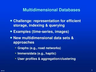
Multidimensional Data Sets & Applications (Examples) • Similarity search, clustering, … • Stock prices time-series • Images color histograms • Shapes angle sequences • Web navigation feature vectors • Spatial & temporal queries, mining queries, … • GeoSpatial data latitude, longitude, altitude • Remote sensory data <lat, long, alt, time, temperature> • Immersidata <x, y, z, t, v>
$price $price f1 e.g., std f2 f5 f (S1) g (S1) 1 1 365 365 day day g (Sn) f (Sn) f3 e.g., avg f4 • A point in 5 dimensions • transformation-based: • FFT, Wavelet [SSDBM’00, 01] • A point in 365 dimensions • (computationally complex) • A point in 2 dimensions • (not accurate enough) Stock Prices S1 Sn
R 255 0 Red Green Blue Red Green Blue . . . 208 125 100 80 100 210 G B More accurate Images Color Histograms j 1 j 2 j 9 j 3 j 8 j 7 j 4 j 5 j 6 Web Navigations Angle Sequences = [j1,j2,j3,j4,j5,j6,j7,j8,j9] P1 P2 P3 P4 P5 … 3 0 8 7 (Hit) Feature Vectors [RIDE’97 … WebKDD’01] More Similarity Search & Clustering C Shapes [ICDE’99 … ICME’00]
Spatial & Temporal Data Complex Queries [ACM-GIS’01, VLDB’01] • Data types: • A point: <latitude, longitude, altitude> or <x, y, z> • A line-segment: <x1, y1, x2, y2> • A line: sequence of line-segments • A region: A closed set of lines • Moving point: <x, y, t> (e.g., car, train, …) • Changing region: <region, value, t> (e.g., changing temperature of a county) • Queries: • Rivers <intersect> Countries • Hospitals <in> Cities • Taxi <within> 5km of Home • <in the next> 10 min • Experiments <overlap> BrainR [Visual’99]
Immersidata and Mining Queries [CIKM’01, UACHI’01]
Immersidata and Mining Queries … … Subject-2 Subject-3 Subject-n … SVD SVD SVD SVD L: A dynamic sign, e.g., ASL colors Subject-1
Avg (sale) d(d <in> 2001) d(s <in> CA) d(p=shoe) Market-Relation Focus Application: On-Line Analytical Processing (OLAP) Market-Relation • Multidimensional data sets: • Dimension attributes (e.g., Store, Product, Data) • Measure attributes (e.g., Sale, Price) • Range-sum queries • Average sale of shoes in CA in 2001 • Number of jackets sold in Seattle in Sep. 2001 • Tougher queries: • Covariance of sale and price of jackets in CA in 2001 (correlation) • Variance of price of jackets in 2001 in Seattle Store Location Date Sale Product Price LA Shoes Jan. 01 $21,500 $85.99 NY Jacket June 01 $28,700 $45.99 . . . . . . . . . . . . . . . Too Slow!
Query: Sum(salary) when (25 < age < 40) and (55k < salary < 150k) Query: Sum(salary) when (25 < age < 40) and (55k < salary < 150k) Traditional Solution: Pre-computation Prefix-sum [Agrawal et. al 1997] Salary Age Age Salary $150k $100k $120k $40k $55k $65k • $50k • $55k • $58k • $100k • $130k • 57 $120k 0 25 40 Age 50 Salary 60 • Disadvantages: • Measure attribute should be pre-selected • Aggregation function should be pre-selected • Works only for limited # of aggregation functions • Updates are expensive (need re-computation) 80 Result: I – II – III + IV
PROPOLYNE: Progressive Evaluationof Polynomial Range-Sum Query (w/ Rolfe Schmidt) • Overview of PROPOLYNE • Features of PROPOLYNE • Polynomial Range-Sum Queries as Vector Queries • Naive Evaluation of Vector Queries Using Wavelets • Fast Evaluation of Vector Queries Using Wavelets • Progressive/Approximate Evaluation of Vector Queries Using Wavelets • Related Work • Performance Results • Conclusion
Overview of PROPOLYNE • Define range-sum query as vector product of query vector and data vector • Offline: Multidimensional wavelet transform of data • At the query time: “lazy” wavelet transform of query vector (very fast) • Dot product of query and data vectors in the transformed domain exact result in O(2 log N)d • Choose high-energy query coefficients only fast approximate result (90% accuracy by retrieving < 10% of data) • Choose query coefficients in order of energy progressive result
PROPOLYNE Features • All attributes can be treated as either “dimension” or “measure” attributes • “Function” can be any polynomial on any combination of attributes, i.e., not only SUM, AVERAGE and COUNT but also COVARIANCE, VARIANCE and SUMSQUARE • Independent from how well the data set can be compressed/approximated by wavelet • Because: We show “range-sum queries” can always be approximated well by wavelets (not always HAAR though!) • Low update cost: O(logd N) • Can be used for exact, approximate and progressiverange-sum query evaluation
Age Salary • $50k • $55k • $58k • $100k • $130k • 57 $120k • Example: F = (Age, Salary) • R:(25 < age < 40) & (55k < salary < 150k) I Polynomial Range-Sum Queries • Polynomial range-sum queries: Q(R,f,I) • I is a finite instance of schema F • RSubSetOf Dom(F), is the range • f : Dom(F) R is a polynomial of degree d
Age Salary • $50k • $55k • $58k • $100k • $130k • 57 $120k I Hence: if where: if Or: Vector Query query data Polynomial Range-Sum Queries as “Vector Queries” • The data frequency distribution of I is the function DI : Dom(F) Z that maps a point x to the number of times it occurs in I • To emphasize the fact that a query is an operator on the data frequency distribution, we write • Example: D(25,50)=D(28,55)=…=D(57,120)=1 and D(x)=0 otherwise.
Summary coefficients of a at level 2 Detail coefficients of a at level 2 a[i]’s Ha[i]’s Ga[i]’s H2a[i]’s GHa[i]’s H3a[i]’s GH2a[i]’s DWT of a Overview of Wavelets H operator: computes a local average of array a at every other point to produce an array of summary coefficients: Ha Example (Haar) h=[1/2,1/2] G operator: measures how much values in the array a vary inside each of the summarized blocks to compute an array of detail coefficients: Ga Example (Haar) g=[1/2,-12] aka wavelet coefficients of a
Naive Evaluation of Vector Queries Using Wavelets • Hence, vector queries can be computed in the wavelet-transformed space as: • Algorithm: • Off-line transformation of data vector (or “data distribution function”, i.e., D, to be exact) • O (|I|ldlogdN) for sparse data, O (|I|) = Nd for dense data • Real-time transformation of the query vector at the query evaluation time • O (ldlogdN) • Sum-up the products of the corresponding elements of data and query vectors • Retrieving elements of data vector: O (Nd)
Ga GH2a GHa Fast Evaluation of Vector Queries Using Wavelets • Main intuitions: • “query vector” can be transformed quickly because most of the coefficients are known in advance • “Transformed query vector” has a large number of negligible (e.g., zero) values (independent on how well data can be approximated by wavelet) • Example: Haar filter & COUNT function on R=[5,12] on the domain of integers from 0 to 15: GH3a H4a At each step, you know the zeros
At boundary of range, summary coeff is ½ *0 + ½ * 1 = ½ Computing Summary Coefficients (Haar Filter, COUNT function) Outside the range, summary coeffs are ½ *0 + ½ * 0 = 0. Inside range, summary coeffs are ½ * 1 + ½ * 1 = 1 The Lazy Wavelet Transform All summary coefficients computed in CONSTANT time! Summary coefficient array looks almost exactly like original array. The only “interesting” activity happens on the boundary.
Computing Detail Coefficients (Haar Filter, COUNT function) Inside range, detail coeffs are ½ * 1 - ½ * 1 = 0 Outside the range, detail coeffs are ½ *0 - ½ * 0 = 0. At lower boundary of range, detail coeff is ½ *0 - ½ * 1 = -½ At upper boundary of range, detail coeff is ½ *1 - ½ * 0 = ½ The Lazy Wavelet Transform All detail coefficients computed in CONSTANT time! All but 2 detail coefficients at each level are equal to zero! The only “interesting” activity happens on the boundary.
Fast Evaluation of Vector Queries Using Wavelets … • Technical Requirements: • Wavelets must satisfy a “moment condition” • Wavelets should have small support (i.e., the shorter the filter, the better) • Supports any Polynomial Range-Sum up to a degree determined by the choice of wavelets • E.g., Haar can only support degree 0 (e.g., COUNT), while db4 can support up to degree 1 (e.g., SUM), and db6 for degree 2 (e.g., VARIANCE) • Standard DWT: O (N) • Our lazy wavelet for transforming query function: O (llog N) where l is the length of the filter
Exact Evaluation of Vector Queries Query: SUM(salary) when (25 < age < 40) & (55k < salary < 150k) # of Wavelet Coefficients: 1250
Name of Technology Research Group Query Cost Update Cost Storage Cost Aggregate Function Support Query Evaluation Support Measure Known at Population? PROPOLYNE 2001 USC Schmidt & Shahabi lg d N(4 )d lg d N(2 )d N d Polynomial Range-Sums of degree Exact, Approximate, Progressive No PROPOLYNE-FM 2001 USC Schmidt & Shahabi 2 d lg d-1 N lg d-1 N N d-1 COUNT and SUM Exact, Approximate, Progressive Yes Space-Efficient Dynamic Data Cube 2000 UCSB El-Abbadi & Agrawal et. al 2 d lg d-1 N lg d-1 N N d-1 COUNT and SUM Exact Yes Relative Prefix-Sum 1999 UCSB 4 d-1 N (d-1)/2 N d-1 COUNT and SUM Exact Yes Prefix-Sum 1997 IBM Agrawal et. al 2 d-1 N d-1 N d-1 COUNT and SUM Exact Yes pCube/MRATree 2000/2001 UCSB and UC Irvine (Mehrota et. al) N d-1 lg N N d COUNT and SUM Exact, Approximate, Progressive Yes Compact Data Cube 1998-2000 Duke and IBM (Vitter et. al) small ? small COUNT and SUM Approximate Yes Optimal Histograms 2001 AT&T (Muthu et. al) small ? small COUNT and SUM Approximate Yes Kernel Density Estimators 1999 Microsoft (Fayyad et. al) small ? small All efficiently computable functions Approximate No
PETROL Data Set: Petroleum sales volume 56504 tuples Five dimensions: <location, product, year, month, volume> Sparseness: 0.16% Traditional data approximation works well 250 range queries generated Randomly from all possible ranges with the uniform dist. Ranges which select fewer than 100 tuples were discarded Median Relative error, Experimental Setup GPS Data Set: • Sensor readings from GPS ground stations in CA • 3358 tuples • Four dimensions: • <lat, long, t, velocity> • Velocity of upward movement of the station • Sparseness: 0.01% • Data approximation works poorly
Performance Results • Compact Data Cube (as a representative of data approximation techniques): under 10% error after using less than 10% of wavelet coefficients (wavelet coefficients sorted in the order of energy) PETROL
Performance Results • CDC needs 5 times as many coefficients as there were tuples in the original table before providing a median relative error of 10% (because data cannot be compressed well) GPS
Conclusion • A novel MOLAP pre-aggregation strategy • Supports conventional aggregates: COUNT, SUM and beyond: COVARIANCE • First pre-aggregation technique that does not require measures be specified a priori • Measures treated as functions of the attributes at the query time • Provides a data independent progressive and approximate query answering technique • With provably poly-logarithmic worst-case query and update costs • And storage cost comparable or better than other pre-aggregation methods
Future • PROPOLYNE future plans: • Use synopsis information about query workloads or data distribution for better sorting of coefficients • Improve random access behavior of PROPOLYNE to data by “clustering” related coeffiecents • More complex queries: OLAP drill-down, general relational algebra queries, … • Multidimensional mining research directions: • Efficient ways of finding trends (e.g., correlation between dimensions/attributes) • Efficient ways of finding surprises/outliers • Mining sequence data sets (e.g., genome databases)