Download
1 / 39
410 likes | 573 Views
Direct Methods for Sparse Linear Systems. Lecture 4 Alessandra Nardi. Thanks to Prof. Jacob White, Suvranu De, Deepak Ramaswamy, Michal Rewienski, and Karen Veroy. Last lecture review. Solution of system of linear equations Existence and uniqueness review Gaussian elimination basics

E N D
Direct Methods for Sparse Linear Systems Lecture 4 Alessandra Nardi Thanks to Prof. Jacob White, Suvranu De, Deepak Ramaswamy, Michal Rewienski, and Karen Veroy
Last lecture review • Solution of system of linear equations • Existence and uniqueness review • Gaussian elimination basics • GE basics • LU factorization • Pivoting
Outline • Error Mechanisms • Sparse Matrices • Why are they nice • How do we store them • How can we exploit and preserve sparsity
Error Mechanisms • Round-off error • Pivoting helps • Ill conditioning (almost singular) • Bad luck: property of the matrix • Pivoting does not help • Numerical Stability of Method
Ill-Conditioning : Norms • Norms useful to discuss error in numerical problems • Norm
Ill-Conditioning : Vector Norms L2 (Euclidean) norm : Unit circle L1 norm : 1 1 L norm : Unit square
Vector induced norm : Ill-Conditioning : Matrix Norms Induced norm of A is the maximum “magnification” of by = max abs column sum = max abs row sum = (largest eigenvalue of ATA)1/2
Ill-Conditioning : Matrix Norms • More properties on the matrix norm: • Condition Number: • It can be shown that: • Large k(A) means matrix is almost singular (ill-conditioned)
Ill-Conditioning: Perturbation Analysis What happens if we perturb b? k(M) large is bad
Ill-Conditioning: Perturbation Analysis What happens if we perturb M? k(M) large is bad Bottom line: If matrix is ill-conditioned, round-off puts you in troubles
Vectors are orthogonal Vectors are nearly aligned Ill-Conditioning: Perturbation Analysis Geometric Approach is more intuitive When vectors are nearly aligned, Hard to decide how much of versus how much of
Numerical Stability • Rounding errors may accumulate and propagate unstably in a bad algorithm. • Can be proven that for Gaussian elimination the accumulated error is bounded
Summary on Error Mechanisms for GE • Rounding: due to machine finite precision we have an error in the solution even if the algorithm is perfect • Pivoting helps to reduce it • Matrix conditioning • If matrix is “good”, then complete pivoting solves any round-off problem • If matrix is “bad” (almost singular), then there is nothing to do • Numerical stability • How rounding errors accumulate • GE is stable
LU – Computational Complexity • Computational Complexity • O(n3), where M: n x n • We cannot afford this complexity • Exploit natural sparsity that occurs in circuits equations • Sparsity: many zero elements • Matrix is sparse when it is advantageous to exploit its sparsity • Exploiting sparsity: O(n1.1) to O(n1.5)
LU – Goals of exploiting sparsity • Avoid storing zero entries • Memory usage reduction • Decomposition is faster since you do need to access them (but more complicated data structure) (2) Avoid trivial operations • Multiplication by zero • Addition with zero (3) Avoid losing sparsity
Sparse Matrices – Resistor Line Tridiagonal Case m
Pivot Multiplier GE Algorithm – Tridiagonal Example For i = 1 to n-1 {“For each Row” For j = i+1 to n {“For each target Row below the source” For k = i+1 to n {“For each Row element beyond Pivot” } } } Order N Operations!
Sparse Matrices – Fill-in – Example 1 Nodal Matrix 0 Symmetric Diagonally Dominant
X X Sparse Matrices – Fill-in – Example 1 Matrix Non zero structure Matrix after one LU step X X X X X= Non zero
X X X X X Sparse Matrices – Fill-in – Example 2 Fill-ins Propagate X X X X X Fill-ins from Step 1 result in Fill-ins in step 2
Fill-ins 0 No Fill-ins 0 Sparse Matrices – Fill-in & Reordering Node Reordering Can Reduce Fill-in - Preserves Properties (Symmetry, Diagonal Dominance) - Equivalent to swapping rows and columns
Exploiting and maintaining sparsity • Criteria for exploiting sparsity: • Minimum number of ops • Minimum number of fill-ins • Pivoting to maintain sparsity: NP-complete problem heuristics are used • Markowitz, Berry, Hsieh and Ghausi, Nakhla and Singhal and Vlach • Choice: Markowitz • 5% more fill-ins but • Faster • Pivoting for accuracy may conflict with pivoting for sparsity
Fill-in Estimate = (Non zeros in unfactored part of Row -1) (Non zeros in unfactored part of Col -1) Markowitz product Sparse Matrices – Fill-in & Reordering Where can fill-in occur ? Already Factored Possible Fill-in Locations Multipliers
Sparse Matrices – Fill-in & Reordering Markowitz Reordering (Diagonal Pivoting) Greedy Algorithm (but close to optimal) !
Sparse Matrices – Fill-in & Reordering Why only try diagonals ? • Corresponds to node reordering in Nodal formulation 1 2 3 1 0 0 3 2 • Reduces search cost • Preserves Matrix Properties - Diagonal Dominance - Symmetry
Sparse Matrices – Fill-in & Reordering Pattern of a Filled-in Matrix Very Sparse Very Sparse Dense
Sparse Matrices – Fill-in & Reordering Unfactored random Matrix
Sparse Matrices – Fill-in & Reordering Factored random Matrix
Sparse Matrices – Data Structure • Several ways of storing a sparse matrix in a compact form • Trade-off • Storage amount • Cost of data accessing and update procedures • Efficient data structure: linked list
Sparse Matrices – Data Structure 1 Orthogonal linked list
Sparse Matrices – Data Structure 2 Vector of row pointers Arrays of Data in a Row Matrix entries Val 11 Val 12 Val 1K 1 Column index Col 11 Col 12 Col 1K Val 21 Val 22 Val 2L Col 21 Col 22 Col 2L Val N1 Val N2 Val Nj N Col N1 Col N2 Col Nj
Sparse Matrices – Data StructureProblem of Misses Eliminating Source Row i from Target row j Row i Row j Must read all the row j entries to find the 3 that match row i Every Miss is an unneeded memory reference (expensive!!!) Could have more misses than ops!
Sparse Matrices – Data Structure Scattering for Miss Avoidance Row j 1) Read all the elements in Row j, and scatter them in an n-length vector 2) Access only the needed elements using array indexing!
Sparse Matrices – Graph Approach Structurally Symmetric Matrices and Graphs 1 X X X X X X X 2 X X X X 3 X X X 4 X X X 5 • One Node Per Matrix Row • One Edge Per Off-diagonal Pair
1 2 X X X X 3 X X X 4 X X X X 5 X X X X X X Sparse Matrices – Graph ApproachMarkowitz Products Markowitz Products = (Node Degree)2
Sparse Matrices – Graph ApproachFactorization One Step of LU Factorization 1 X X X X X X X 2 X X X X X 3 X X X 4 X X X X X 5 • Delete the node associated with pivot row • “Tie together” the graph edges
1 2 3 4 5 1 2 3 4 5 Sparse Matrices – Graph ApproachExample Graph Markowitz products ( = Node degree)
1 3 4 5 Sparse Matrices – Graph ApproachExample Swap 2 with 1 Graph
Summary • Gaussian Elimination Error Mechanisms • Ill-conditioning • Numerical Stability • Gaussian Elimination for Sparse Matrices • Improved computational cost: factor in O(N1.5) operations (dense is O(N3) ) • Example: Tridiagonal Matrix Factorization O(N) • Data structure • Markowitz Reordering to minimize fill-ins • Graph Based Approach