Download

1 / 57
570 likes | 663 Views
The Frequency Domain. Somewhere in Cinque Terre, May 2005. 15-463: Computational Photography Alexei Efros, CMU, Fall 2011. Many slides borrowed from Steve Seitz. Salvador Dali “Gala Contemplating the Mediterranean Sea, which at 30 meters becomes the portrait of Abraham Lincoln ”, 1976.

E N D
The Frequency Domain Somewhere in Cinque Terre, May 2005 15-463: Computational Photography Alexei Efros, CMU, Fall 2011 Many slides borrowed from Steve Seitz
Salvador Dali “Gala Contemplating the Mediterranean Sea, which at 30 meters becomes the portrait of Abraham Lincoln”, 1976 Salvador Dali, “Gala Contemplating the Mediterranean Sea, which at 30 meters becomes the portrait of Abraham Lincoln”, 1976 Salvador Dali, “Gala Contemplating the Mediterranean Sea, which at 30 meters becomes the portrait of Abraham Lincoln”, 1976
A nice set of basis Teases away fast vs. slow changes in the image. This change of basis has a special name…
Jean Baptiste Joseph Fourier (1768-1830) had crazy idea (1807): Any univariate function can be rewritten as a weighted sum of sines and cosines of different frequencies. Don’t believe it? Neither did Lagrange, Laplace, Poisson and other big wigs Not translated into English until 1878! But it’s (mostly) true! called Fourier Series there are some subtle restrictions ...the manner in which the author arrives at these equations is not exempt of difficulties and...his analysis to integrate them still leaves something to be desired on the score of generality and even rigour. Laplace Legendre Lagrange
A sum of sines • Our building block: • Add enough of them to get any signal f(x) you want! • How many degrees of freedom? • What does each control? • Which one encodes the coarse vs. fine structure of the signal?
Inverse Fourier Transform Fourier Transform F(w) f(x) F(w) f(x) Fourier Transform • We want to understand the frequency w of our signal. So, let’s reparametrize the signal by w instead of x: • For every w from 0 to inf, F(w) holds the amplitude A and phase f of the corresponding sine • How can F hold both? Complex number trick! We can always go back:
Time and Frequency • example : g(t) = sin(2pf t) + (1/3)sin(2p(3f) t)
Time and Frequency • example : g(t) = sin(2pf t) + (1/3)sin(2p(3f) t) = +
Frequency Spectra • example : g(t) = sin(2pf t) + (1/3)sin(2p(3f) t) = +
Frequency Spectra • Usually, frequency is more interesting than the phase
Frequency Spectra = + =
Frequency Spectra = + =
Frequency Spectra = + =
Frequency Spectra = + =
Frequency Spectra = + =
Extension to 2D in Matlab, check out: imagesc(log(abs(fftshift(fft2(im)))));
Fourier analysis in images Intensity Image Fourier Image http://sharp.bu.edu/~slehar/fourier/fourier.html#filtering
Signals can be composed + = http://sharp.bu.edu/~slehar/fourier/fourier.html#filtering More: http://www.cs.unm.edu/~brayer/vision/fourier.html
The greatest thing since sliced (banana) bread! The Fourier transform of the convolution of two functions is the product of their Fourier transforms The inverse Fourier transform of the product of two Fourier transforms is the convolution of the two inverse Fourier transforms Convolution in spatial domain is equivalent to multiplication in frequency domain! The Convolution Theorem
2D convolution theorem example |F(sx,sy)| f(x,y) * h(x,y) |H(sx,sy)| g(x,y) |G(sx,sy)|
Filtering Gaussian Box filter Why does the Gaussian give a nice smooth image, but the square filter give edgy artifacts?
Low-pass, Band-pass, High-pass filters low-pass: High-pass / band-pass:
What does blurring take away? original
What does blurring take away? smoothed (5x5 Gaussian)
High-Pass filter smoothed – original
Band-pass filtering • Laplacian Pyramid (subband images) • Created from Gaussian pyramid by subtraction Gaussian Pyramid (low-pass images)
Laplacian Pyramid • How can we reconstruct (collapse) this pyramid into the original image? Need this! Original image
Why Laplacian? Gaussian Laplacian of Gaussian delta function
Project 1g: Hybrid Images unit impulse Laplacian of Gaussian Gaussian Gaussian Filter! Laplacian Filter! A. Oliva, A. Torralba, P.G. Schyns, “Hybrid Images,” SIGGRAPH 2006 Project Instructions: http://www.cs.illinois.edu/class/fa10/cs498dwh/projects/hybrid/ComputationalPhotography_ProjectHybrid.html
Clues from Human Perception Early processing in humans filters for various orientations and scales of frequency Perceptual cues in the mid frequencies dominate perception When we see an image from far away, we are effectively subsampling it Early Visual Processing: Multi-scale edge and blob filters
Frequency Domain and Perception Campbell-Robson contrast sensitivity curve
- = + a = Unsharp Masking
Lossy Image Compression (JPEG) Block-based Discrete Cosine Transform (DCT)
Using DCT in JPEG The first coefficient B(0,0) is the DC component, the average intensity The top-left coeffs represent low frequencies, the bottom right – high frequencies
Image compression using DCT Quantize More coarsely for high frequencies (which also tend to have smaller values) Many quantized high frequency values will be zero Encode Can decode with inverse dct Filter responses Quantization table Quantized values
JPEG Compression Summary http://en.wikipedia.org/wiki/YCbCr http://en.wikipedia.org/wiki/JPEG Subsample color by factor of 2 • People have bad resolution for color Split into blocks (8x8, typically), subtract 128 For each block • Compute DCT coefficients for • Coarsely quantize • Many high frequency components will become zero • Encode (e.g., with Huffman coding)
Block size in JPEG Block size small block faster correlation exists between neighboring pixels large block better compression in smooth regions It’s 8x8 in standard JPEG
JPEG compression comparison 89k 12k