Download
1 / 18
180 likes | 407 Views
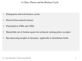
6. Chaos-Theory and the Business Cycle. Endogenous and real business cycles Derived from natural sciences Flourished in 1980s and 1990s Meanwhile out of fashion again ( too technical , lacking policy receipts )

E N D
6. Chaos-Theory and the Business Cycle • Endogenousand real businesscycles • Derivedfromnaturalsciences • Flourished in 1980s and 1990s • Meanwhile out offashionagain (tootechnical, lackingpolicyreceipts) • But interestinginsights in dynamics, applicabletodistribution-battle 1 U van Suntum, Vorlesung KuB 1
Chaos-theory: An example*) x t+1 = r xt(1 – xt) Xmax = 0,25 r x t+1 xt 0 0,5 1,0 *) cf. Ian Stewart, Spielt Gott Roulette? Chaos in der Mathematik, Basel u.a. 1990, S. 163 ff.; Heubes, Konjunktur u. Wachstum, a.a.O., S. 108 KuKuB 7 2 KuB 7 U van Suntum, Vorlesung KuB 2
Derivation of maximum: x t+1 = r xt(1 – xt) Xmax = 0,25 r x t+1 0,5 xt 3 KuB 7 U van Suntum, Vorlesung KuB 3
Derivation of fixed point (equlibrium): x t+1 = r xt (1 – xt) 45o x t+1 = xt Xmax = 0,25 r x t+1 „fixed point“ 0,5 xt Existenceofequilibriumis not sufficienttoguaranteeitsfeasibilityandstability! 4 KuB 7 U van Suntum, Vorlesung KuB 4
x t+1 = r xt (1 – xt) Y t+1 = aYt (1 – Yt) • with 0 < r < 3 => convergence to fixed point • with 3 < r < 3,58 => fluctuations (bifurcations) • with 3,58 < r < 4 => chaos with occasional periodicity • with r > 4 => exploding Chaosgleichungbeispiel.xls Fixed point (stable if absolute slope of curve < 1) Xmax = 0,25 r x t+1 45o Points which are feasible in principle xt Startwert 5 KuB 7 U van Suntum, Vorlesung KuB 5
a) convergence (0 < r < 3); here: r = 2,8 => fixed point = 0,6428 fixed point: x = 0,6428 start: x = 0,4 temporal behavior of x 6 KuB 7 U van Suntum, Vorlesung KuB 6
b) bifurcations (3 < r < 3,58); here: r = 3,2 => fixed point = 0,6875 points of bifurcation:*) x = 0, 7995 und x = 0,5130 start: x = 0,4 *) numericallyderived by Excel-Solver: conditions: x t+1 = x t+3 and x t+2 = x t+4 temporal behavior of x 7 KuB 7 U van Suntum, Vorlesung KuB 7
c) chaos (3,58 < r < 4); here: r = 3,8 => fixed point = 0,7368 start: x = 0,4 temporal behavior of x 8 KuB 7 U van Suntum, Vorlesung KuB 8
d) explosion ( r > 4); here: r = 4,2 start: x = 0,4 temporal behavior of x 9 KuB 7 U van Suntum, Vorlesung KuB 9
Economic application: Goodwin/Pohjola-model (1967/1981) (cf. Heubes, Konjunktur und Wachstum) • wages w (and wage share u = W/Y) rise in Y • grwoth rate gY declines in wage share u (1 – u) g u u g (1 – u) 10 KuB 7 U van Suntum, Vorlesung KuB 10
Application: Business Cycle Model of Goodwin/Pohjola (1967/1981) • Assumptions: • Leontief production function=> g denotes growth rate of Y, K and N • Classical saving function: amount G is saved, amount W consumed • Additional simplifications here: no technical progress, size of labor force fixed • Wages increase in employment and labor productivity Variables: I = investment, K = capital stock, N= labor, k = capital coefficient K/Y, w = wage rate , d = wage adjustment parameter, N* = equilibrium employment (fixed point of chaos model) 11 KuB 7 U van Suntum, Vorlesung KuB 11
Formal Derivation of Goodwin/Pohjola-Model chaos with k < 0,39 KuB 7 U van Suntum, Vorlesung KuB 12 12
Chaosgleichungbeispiel.xls • Explanation: • investment proportional to profit share (1-u) because all profits are saved (eq.1) • employment proportional to total income because of Leontief PF (eq. 2) • high employment and high productivity increase wage rate (eq. 3) • model culminates in a single difference equation (eq. 6, 7). • thus with given starting point N and constant N* employment is determined at any t • empirical estimation by autoregressive methods (using only Nt, Nt-1 etc.) KuKuB 7 13 KuB 7 U van Suntum, Vorlesung KuB 13
Grafical exposition with k < 0,39 (here: k = 0,38) employment N(t) KuKuB 7 14 KuB 7 U van Suntum, Vorlesung KuB 14
bifurcation with k > 0,4 (here: k = 0,6) Damped fluctuations with k >> 0,4 (here: k = 0,6) employment N(t) employment N(t) Summary: anything goes… 15 KuB 7 U van Suntum, Vorlesung KuB 15
Strengths: Shows dynamics of business cycle Easily transformable into econometrics Can explain erratic fluctuations Weaknesses: technical, relatively little economic content Poor policy relevance Very simple economic model Critique of Chaos-Theory 16 KuB 7 U van Suntum, Vorlesung KuB 16
How do mathematicans and economists define chaos? What is the fixed point of a dynamic model? What are bifurcations? Where do the dynamics in the Goodwin/Pohjola model come from? How does the wage share behave over the business cycle? Lerning goals/Questions 17 KuB 7 U van Suntum, Vorlesung KuB 17
Exercise: Assume the following difference equation for total demand in the business cycle: • Letparameter a be 4.20 • Whatisthemaximumpossiblevalueof Y? • Whatisthefixedpointofthe model? KuKuB 7 18 KuB 7