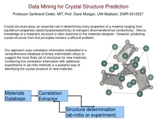
Data Mining for Protein Structure Prediction
Data Mining for Protein Structure Prediction. Mohammed J. Zaki SPIDER Data Mining Project: S calable, P arallel and I nteractive D ata Mining and E xploration at R PI http://www.cs.rpi.edu/~zaki. Outline of the Talk. How do proteins form? Protein folding problem Contact map mining

Data Mining for Protein Structure Prediction
E N D
Presentation Transcript
Data Mining for Protein Structure Prediction Mohammed J. Zaki SPIDER Data Mining Project: Scalable, Parallel and Interactive Data Mining and Exploration at RPI http://www.cs.rpi.edu/~zaki
Outline of the Talk • How do proteins form? • Protein folding problem • Contact map mining • Using HMMs based on local motifs • Mining “physical” dense frequent patterns (non-local motifs) • Future directions • Heuristic rules • Folding pathways
How do Proteins Form? • Building Blocks of Biological Systems • DNA (nucleotides, 4 types): information carrier/encoder • RNA: bridge from DNA to protein • Protein (amino acids, 20 types): action molecules. • Processes • Replication of DNA • Transcription of gene (DNA) to messenger RNA (mRNA) • Splicing of non-coding regions of the genes (introns) • Translation of mRNA into proteins • Folding of proteins into 3D structure • Biochemical or structural functions of proteins
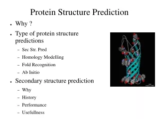
Protein Structures • Primary structure • Un-branched polymer • 20 side chains (residues or amino acids) • Higher order structures • Secondary: local (consecutive) in sequence • Tertiary: 3D fold of one polypeptide chain • Quaternary: Chains packing together
Contact Map • Amino acids Ai and Aj are in contact if their 3D distance is less than threshold (7å) • Sequence separation is given as |i-j| • Contact map C is an N x N matrix, where • C(i,j) = 1 if Ai and Aj are in contact • C(i,j) = 0 otherwise • Consider all pairs with |i-j| >= 4
Protein 2igd: 3D Structure Anti-parallel Beta Sheets Alpha Helix Parallel Beta Sheets
Contact Map (2igd PDB) Parallel Beta Sheets Anti-parallel Beta Sheets Alpha Helix Amino Acid Aj Amino Acid Ai
How much information in Amino Acids Alone: Classification Problem • A pair of amino acids (Ai,Aj) is an instance • The class: C (1) or NC (0), i.e., contact or non-contact • Highly skewed class distribution • 1.7% C and 98.3% NC; 300K C vs 17,3M NC • Features for each instance • Ai and Aj • Class: C or NC
Predicting Protein Contacts • Predict contacts for new sequence
Classification via Association Mining • Association mining good for skewed data • Mining: Mine frequent itemsets in C data (Dc) • P(X | Dc) = Frequency(X | Dc) / |Dc| • Counting: find P(X | Dnc) • Pruning • Likelihood of a contact: r = P(X|Dc) / P(X|Dnc) • Prune pattern X if ratio r of contact to non-contact probability is less then some threshold • i.e., keep only the patterns highly predictive of contacts
Testing Phase • 90-10 split into training and testing • 2.4 million pairs, with 36K contacts (1.5%) • Evidence calculation: • Find matching patterns P for each instance • Compute cumulative frequency in C and NC • Sc = Sum of frequency (X | Dc) where X in P • Snc = Sum of frequency (X | Dnc) where X in P • Compute evidence: ratio of Sc / Snc • Prediction: Sort instances on evidence • Predict top PR fraction as contacts
Experiments • 794 Proteins from Protein Data Bank • Distinct structures (< 25% similarity) • Longest: 907, Smallest: 35 amino acids • 90-10 split for training-testing • Total pairs: 20 million (> 2.5 GB) • Contacts: 330 thousand (1.6%) • Highly uneven class distribution
Evaluation Metrics • Na: set of all pairs • Na*: all pairs with positive evidence • Ntc: true contacts in test data • Ntc*: true contacts with positive evidence • Npc: predicted contacts • Ntpc: correctly predicted contacts • Accuracy = Ntpc / Npc • Coverage = Ntpc / Ntc • Prediction Ratio (PR): Ntc*/Na* • Random Predictor Accuracy: Ntc/Na
Results (Amino Acids; All Lengths) Crossover: 7% accuracy and 7% coverage; 2 times over Random
Results (Amino Acids; by length) 1-100: 12% accuracy(A) and coverage (C); 100-170: 6% A and C 170-300: 4.5% A and C; 300+: 2% A and C
An HMM for Local Predictions • HMMSTR (Chris Bystroff, Biology, RPI) • Build a library of short sequences that tend to fold uniquely across protein families: the I-Sites Library • Treat each motif as a Markov chain • Merge the motifs into a global HMM for local structure prediction
Training the HMM • Build I-sites Library • Short sequence motifs (3 to 19) • Exhaustive clustering of sequences • Non-redundant PDB dataset (< 25% similarity) • Build an HMM • Each of 262 motifs is a chain of Markov states • Each state has sequence and structure for one position • Merge I-sites motifs hierarchically to get one global HMM for all the motifs
HMM Output • Total of 282 States in the HMM • Each state produces or “emits”: • Amino acid profile (20 probability values) • Secondary structure (D) (helix, strand or loop) • Backbone angles (R) (11 dihedral angle symbols) • Finer structural context (C) (10 context symbols)
I-Sites Motifs (Initiation Sites) Beta Hairpin Beta to Alpha Helix C-Cap
Data Format and Preparation • Take the 794 PDB proteins • Compute optimal alignment to HMM • Find best state sequence for the observed acids • Output probability distribution of a residue over all the 282 HMM states • Integrate the 3 datasets • Alignment probability distribution (Nx282) • Amino acid and context information (D, R, C) • Contact map (NxN)
Adding features from HMMSTR • The class: C (1) or NC (0) • Highly skewed class distribution • Approx 1.5% C and 98.5% NC • Features for each instance • Ai Aj Di Dj Ri Rj Ci Cj • Profile: pi1 pi2 … pi20 pj1 pj2 … pj20 • HMM States: qi1 qi2 .. qi282 qj1 qj2 .. qj282 • Class: C or NC
HMM and AA + (R,D,C) ; All Lengths Left Crossover: 19% accuracy and coverage; 5.3 times over Random Right Crossover (+RDC): 17% accuracy and coverage; 5 times over Random
HMM + AA + R,D,C (by length) 1-100: 30% accuracy(A) and coverage (C); 100-170: 17% A and C 170-300: 10% A and C; 300+: 6% A and C
Summary of Classification Results • Challenging prediction problem • In essence, we have to predict a contact matrix for a new protein • Hybrid HMM/Associations approach • Best results to-date: 19% overall accuracy/coverage, 30% for short proteins • 14.4% Accuracy (Fariselli, Casadio ‘99; NN) • 13% Accuracy (Thomas et al ‘96) • Short proteins: 26% (Olmea, Valencia, ‘97)
Mining “Physical” Dense Frequent Patterns (non-local motifs)
Characterizing Physical, Protein-like Contact Maps • A very small subset of all contact maps code for physically possible proteins (self-avoiding, globular chains) • A contact map must: • Satisfy geometric constraints • Represent low-energy structure • What are the typical non-local interactions? • Frequent dense 0/1 submatrices in contact maps • 3-step approach: 1) data generation, 2) dense pattern mining, and 3) mapping to structure space
Dense Pattern Mining • 12,524 protein-like 60 residue structures • Use HMMSTR to generate protein-like sequences • Use ROSETTA to generate their structures • Monte Carlo fragment insertion (from I-sites library) • Up to 5 possible low-energy structures retained • Frequent 2D Pattern Mining • Use WxW sliding window; W window size • Measure density under each window • (N-W)^2 / 2 possible windows per N length protein • Look for “minimum density”; scale away from diag • Try different window sizes
Counting Dense Patterns • Naïve Approach:for W=5, N=60 there are 1485 windows per protein. Total 15 Million possible windows for 12,524 proteins • Test if two submatrices are equal • Linear search: O(P x W^2) with P current dense patterns • Hash based: O(W^2) • Our Approach: 2-level Hashing • O(W) time
Pattern (WxW Submatrix) Encoding • Encode submatrix as string (W integers) Submatrix Integer Value 00000 0 01100 12 01000 8 01000 8 00000 0 Concatenated String: 0.12.8.8.0
Two-level Hashing • String ID (M) = • Level 1 (approximate): • Level2 (exact) : h2 (M) = StringID (M)
Binding Patterns to Proteins Sequence and Structure • Using window size, W=5 • StringID:0.12.8.8.0, Support = 170 00000 01100 01000 01000 00000 • Occurrences: pdb-name (X,Y) X_sequence Y_sequence Interaction 1070.0 52,30 ILLKN TFVRI alpha::beta 1145.0 51,13 VFALH GFHIA alpha::strand 1251.2 42,6 EVCLR GSKFG alpha::strand 1312.0 54,11 HGYDE ATFAK alpha::beta 1732.0 49,6 HRFAK KELAG alpha::beta 2895.0 49,7 SRCLD DTIYY alpha::beta ...
Frequent Dense Non-Local Patterns Alpha – Alpha Alpha – Beta Sheet
Frequent Dense Non-Local Patterns Alpha – Beta Turn Beta Sheet – Beta Turn