Reinforcement Learning

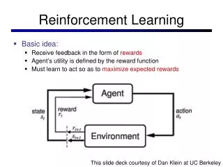
Reinforcement Learning • Basic idea: • Receive feedback in the form of rewards • Agent’s utility is defined by the reward function • Must learn to act so as to maximize expected rewards This slide deck courtesy of Dan Klein at UC Berkeley

Grid World • The agent lives in a grid • Walls block the agent’s path • The agent’s actions do not always go as planned: • 80% of the time, the action North takes the agent North (if there is no wall there) • 10% of the time, North takes the agent West; 10% East • If there is a wall in the direction the agent would have been taken, the agent stays put • Small “living” reward each step • Big rewards come at the end • Goal: maximize sum of rewards*

Markov Decision Processes • An MDP is defined by: • A set of states s  S • A set of actions a  A • A transition function T(s,a,s’) • Prob that a from s leads to s’ • i.e., P(s’ | s,a) • Also called the model • A reward function R(s, a, s’) • Sometimes just R(s) or R(s’) • A start state (or distribution) • Maybe a terminal state • MDPs are a family of non-deterministic search problems • Reinforcement learning: MDPs where we don’t know the transition or reward functions

What is Markov about MDPs? • Andrey Markov (1856-1922) • “Markov” generally means that given the present state, the future and the past are independent • For Markov decision processes, “Markov” means:

Solving MDPs • In deterministic single-agent search problems, want an optimal plan, or sequence of actions, from start to a goal • In an MDP, we want an optimal policy *: S → A • A policy  gives an action for each state • An optimal policy maximizes expected utility if followed • Defines a reflex agent Optimal policy when R(s, a, s’) = -0.03 for all non-terminals s

Example Optimal Policies R(s) = -0.01 R(s) = -0.03 R(s) = -0.4 R(s) = -2.0

Example: High-Low • Three card types: 2, 3, 4 • Infinite deck, twice as many 2’s • Start with 3 showing • After each card, you say “high” or “low” • New card is flipped • If you’re right, you win the points shown on the new card • Ties are no-ops • If you’re wrong, game ends • Differences from expectimax: • #1: get rewards as you go • #2: you might play forever! 3 4 2 2

High Low 3 3 , High , Low T = 0.25, R = 3 T = 0, R = 4 T = 0.25, R = 0 T = 0.5, R = 2 3 2 4 High Low High Low Low High Example: High-Low 3

MDP Search Trees • Each MDP state gives an expectimax-like search tree s is a state s a (s, a) is a q-state s, a (s,a,s’) called a transition T(s,a,s’) = P(s’|s,a) R(s,a,s’) s,a,s’ s’

Utilities of Sequences • In order to formalize optimality of a policy, need to understand utilities of sequences of rewards • Typically consider stationary preferences: • Theorem: only two ways to define stationary utilities • Additive utility: • Discounted utility:

Infinite Utilities?! • Problem: infinite state sequences have infinite rewards • Solutions: • Finite horizon: • Terminate episodes after a fixed T steps (e.g. life) • Gives nonstationary policies ( depends on time left) • Absorbing state: guarantee that for every policy, a terminal state will eventually be reached (like “done” for High-Low) • Discounting: for 0 <  < 1 • Smaller  means smaller “horizon” – shorter term focus

Discounting • Typically discount rewards by  < 1 each time step • Sooner rewards have higher utility than later rewards • Also helps the algorithms converge

s a s, a s,a,s’ s’ Recap: Defining MDPs • Markov decision processes: • States S • Start state s0 • Actions A • Transitions P(s’|s,a) (or T(s,a,s’)) • Rewards R(s,a,s’) (and discount ) • MDP quantities so far: • Policy = Choice of action for each state • Utility (or return) = sum of discounted rewards

s a s, a s,a,s’ s’ Optimal Utilities • Fundamental operation: compute the values (optimal expectimax utilities) of states s • Why? Optimal values define optimal policies! • Define the value of a state s: V*(s) = expected utility starting in s and acting optimally • Define the value of a q-state (s,a): Q*(s,a) = expected utility starting in s, taking action a and thereafter acting optimally • Define the optimal policy: *(s) = optimal action from state s

s a s, a s,a,s’ s’ The Bellman Equations • Definition of “optimal utility” leads to a simple one-step lookahead relationship amongst optimal utility values: Optimal rewards = maximize over first action and then follow optimal policy • Formally:

s a s, a s,a,s’ s’ Solving MDPs • We want to find the optimal policy* • Proposal 1: modified expectimax search, starting from each state s:

Why Not Search Trees? • Why not solve with expectimax? • Problems: • This tree is usually infinite (why?) • Same states appear over and over (why?) • We would search once per state (why?) • Idea: Value iteration • Compute optimal values for all states all at once using successive approximations • Will be a bottom-up dynamic program similar in cost to memoization • Do all planning offline, no replanning needed!

Value Estimates • Calculate estimates Vk*(s) • Not the optimal value of s! • The optimal value considering only next k time steps (k rewards) • As k  , it approaches the optimal value • Why: • If discounting, distant rewards become negligible • If terminal states reachable from everywhere, fraction of episodes not ending becomes negligible • Otherwise, can get infinite expected utility and then this approach actually won’t work

Value Iteration • Idea: • Start with V0*(s) = 0, which we know is right (why?) • Given Vi*, calculate the values for all states for depth i+1: • This is called a value update or Bellman update • Repeat until convergence • Theorem: will converge to unique optimal values • Basic idea: approximations get refined towards optimal values • Policy may converge long before values do

Example: =0.9, living reward=0, noise=0.2 Example: Bellman Updates max happens for a=right, other actions not shown

Example: Value Iteration V2 V3 • Information propagates outward from terminal states and eventually all states have correct value estimates

Convergence* • Define the max-norm: • Theorem: For any two approximations U and V • I.e. any distinct approximations must get closer to each other, so, in particular, any approximation must get closer to the true U and value iteration converges to a unique, stable, optimal solution • Theorem: • I.e. once the change in our approximation is small, it must also be close to correct

MDP Search Trees • Each MDP state gives an expectimax-like search tree s is a state s a (s, a) is a q-state s, a (s,a,s’) called a transition T(s,a,s’) = P(s’|s,a) R(s,a,s’) s,a,s’ s’

Practice: Computing Actions • Which action should we chose from state s: • Given optimal values V? • Given optimal q-values Q? • Lesson: actions are easier to select from Q’s!

Utilities for Fixed Policies • Another basic operation: compute the utility of a state s under a fix (general non-optimal) policy • Define the utility of a state s, under a fixed policy : V(s) = expected total discounted rewards (return) starting in s and following  • Recursive relation (one-step look-ahead / Bellman equation): s (s) s, (s) s, (s),s’ s’

Policy Evaluation • How do we calculate the V’s for a fixed policy? • Idea one: modify Bellman updates • Idea two: it’s just a linear system, solve with Matlab (or whatever)

Policy Iteration • Problem with value iteration: • Considering all actions each iteration is slow: takes |A| times longer than policy evaluation • But policy doesn’t change each iteration, time wasted • Alternative to value iteration: • Step 1: Policy evaluation: calculate utilities for a fixed policy (not optimal utilities!) until convergence (fast) • Step 2: Policy improvement: update policy using one-step lookahead with resulting converged (but not optimal!) utilities (slow but infrequent) • Repeat steps until policy converges • This is policy iteration • It’s still optimal! • Can converge faster under some conditions

Policy Iteration • Policy evaluation: with fixed current policy , find values with simplified Bellman updates: • Iterate until values converge • Policy improvement: with fixed utilities, find the best action according to one-step look-ahead

Comparison • In value iteration: • Every pass (or “backup”) updates both utilities (explicitly, based on current utilities) and policy (possibly implicitly, based on current policy) • In policy iteration: • Several passes to update utilities with frozen policy • Occasional passes to update policies • Hybrid approaches (asynchronous policy iteration): • Any sequences of partial updates to either policy entries or utilities will converge if every state is visited infinitely often

Reinforcement Learning • Reinforcement learning: • Still have an MDP: • A set of states s  S • A set of actions (per state) A • A model T(s,a,s’) • A reward function R(s,a,s’) • Still looking for a policy (s) • New twist: don’t know T or R • I.e. don’t know which states are good or what the actions do • Must actually try actions and states out to learn [DEMO]

Example: Animal Learning • RL studied experimentally for more than 60 years in psychology • Rewards: food, pain, hunger, drugs, etc. • Mechanisms and sophistication debated • Example: foraging • Bees learn near-optimal foraging plan in field of artificial flowers with controlled nectar supplies • Bees have a direct neural connection from nectar intake measurement to motor planning area

Example: Backgammon • Reward only for win / loss in terminal states, zero otherwise • TD-Gammon learns a function approximation to V(s) using a neural network • Combined with depth 3 search, one of the top 3 players in the world • You could imagine training Pacman this way… • … but it’s tricky! (It’s also P3)

Reinforcement Learning