Totally Unimodular Matrices
270 likes | 523 Views
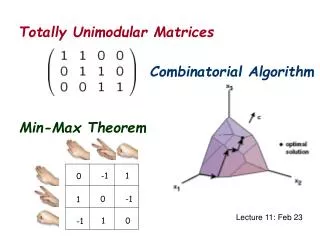
-1. 1. 0. 0. -1. 1. 1. 0. -1. Totally Unimodular Matrices. Combinatorial Algorithm . Min-Max Theorem . Lecture 11: Feb 23. 2 Player Game. Column player. -1. 1. 0. Strategy: A probability distribution. Row player. 0. -1. 1. 1. 0. -1.

Totally Unimodular Matrices
E N D
Presentation Transcript
-1 1 0 0 -1 1 1 0 -1 Totally Unimodular Matrices Combinatorial Algorithm Min-Max Theorem Lecture 11: Feb 23
2 Player Game Column player -1 1 0 Strategy: A probability distribution Row player 0 -1 1 1 0 -1 Row player tries to maximize the payoff, column player tries to minimize
2 Player Game Column player Strategy: A probability distribution Row player A(i,j) You have to decide your strategy first. Is it fair??
Von Neumann Minimax Theorem Strategy set Which player decides first doesn’t matter! e.g. paper, scissor, rock.
Key Observation If the row player fixes his strategy, then we can assume that y chooses a pure strategy Vertex solution is of the form (0,0,…,1,…0), i.e. a pure strategy
Key Observation similarly
Primal Dual Programs duality
Other Applications • Analysis of randomized algorithms (Yao’s principle) • Cost sharing • Price setting
Totally Unimodular Matrices m constraints, n variables Vertex solution: unique solution of n linearly independent tight inequalities Can be rewritten as: That is:
Totally Unimodular Matrices Assuming all entries of A and b are integral When does has an integral solution x? By Cramer’s rule where Ai is the matrix with each column is equal to the corresponding column in A except the i-th column is equal to b. x would be integral if det(A) is equal to +1 or -1.
Totally Unimodular Matrices A matrix is totally unimodular if the determinant of each square submatrix of is 0, -1, or +1. Theorem 1: If A is totally unimodular, then every vertex solution of is integral. Proof (follows from previous slides): • a vertex solution is defined by a set of n linearly independent tight inequalities. • Let A’ denote the (square) submatrix of A which corresponds to those inequalities. • Then A’x = b’, where b’ consists of the corresponding entries in b. • Since A is totally unimodular, det(A) = 1 or -1. • By Cramer’s rule, x is integral.
Example of Totally Unimodular Matrices A totally unimodular matrix must have every entry equals to +1,0,-1. Guassian elimination And so we see that x must be an integral solution.
Example of Totally Unimodular Matrices is not a totally unimodular matrix, as its determinant is equal to 2. x is not necessarily an integral solution.
Totally Unimodular Matrices Primal Dual Transpose of A Theorem 2: If A is totally unimodular, then both the primal and dual programs are integer programs. Proof: if A is totally unimodular, then so is it’s transpose.
Application 1: Bipartite Graphs Let A be the incidence matrix of a bipartite graph. Each row i represents a vertex v(i), and each column j represents an edge e(j). A(ij) = 1 if and only if edge e(j) is incident to v(i). edges vertices
Application 1: Bipartite Graphs We’ll prove that the incidence matrix A of a bipartite graph is totally unimodular. Consider an arbitrary square submatrix A’ of A. Our goal is to show that A’ has determinant -1,0, or +1. Case 1: A’ has a column with only 0. Then det(A’)=0. Case 2: A’ has a column with only one 1. By induction, A’’ has determinant -1,0, or +1. And so does A’.
Application 1: Bipartite Graphs Case 3: Each column of A’ has exactly two 1. +1 We can write -1 Since the graph is bipartite, each column has one 1 in Aup and one 1 in Adown So, by multiplying +1 on the rows in Aup and -1 on the columns in Adown, we get that the rows are linearly dependent, and thus det(A’)=0, and we’re done. +1 -1
Application 1: Bipartite Graphs Maximum bipartite matching Incidence matrix of a bipartite graph, hence totally unimodular, and so yet another proof that this LP is integral.
Application 1: Bipartite Graphs Maximum general matching The linear program for general matching does not come from a totally unimodular matrix, and this is why Edmonds’ result is regarded as a major breakthrough.
Application 1: Bipartite Graphs Theorem 2: If A is totally unimodular, then both the primal and dual programs are integer programs. Maximum matching <= maximum fractional matching <= minimum fractional vertex cover <= minimum vertex cover Theorem 2 show that the first and the last inequalities are equalites. The LP-duality theorem shows that the second inequality is an equality. And so we have maximum matching = minimum vertex cover.
Application 2: Directed Graphs • Let A be the incidence matrix of a directed graph. • Each row i represents a vertex v(i), • and each column j represents an edge e(j). • A(ij) = +1 if vertex v(i) is the tail of edge e(j). • A(ij) = -1 if vertex v(i) is the head of edge e(j). • A(ij) = 0 otherwise. The incidence matrix A of a directed graph is totally unimodular. • Consequences: • The max-flow problem (even min-cost flow) is polynomial time solvable. • Max-flow-min-cut theorem follows from the LP-duality theorem.
Simplex Method • Simplex Algorithm: • Start from an arbitrary vertex. • Move to one of its neighbours • which improves the cost. Iterate. For combinatorial problems, we know that vertex solutions correspond to combinatorial objects like matchings, stable matchings, flows, etc. So, the simplex algorithm actually defines a combinatorial algorithm for these problems.
Simplex Method For example, if you consider the bipartite matching polytope and run the simplex algorithm, you get the augmenting path algorithm. The key is to show that two adjacent vertices are differed by an augmenting path. Recall that a vertex solution is the unique solution of n linearly independent inequalities. So, moving along an edge in the polytope means to replace one tight inequality by another one. There is one degree of freedom and this corresponds to moving along an edge.
Summary How to model a combinatorial problem as a linear program. See the geometric interpretation of linear programming. How to prove a linear program gives integer optimal solutions? • Prove that every vertex solution is integral. • By convex combination method. • By linear independency of tight inequalities. • By totally unimodular matrices. • By shifting technique.
Polynomial Time Solvable Problems Stable matchings Bipartite matchings Weighted Bipartite matchings General matchings Maximum flows Shortest paths Minimum spanning trees Minimum Cost Flows Matroid intersection Graph orientation Submodular Flows Packing directed trees Connectivity augmentation Linear programming
Summary How to obtain min-max theorems of combinatorial problems? LP-duality theorem, e.g. max-flow-min-cut, max-matching-min-vertex-cover. See combinatorial algorithms from the simplex algorithm, and even give an explanation for the combinatorial algorithms (local minimum = global minimum).
![[MATRICES ]](https://cdn4.slideserve.com/144276/matrices-dt.jpg)