Chapter 22: Advanced Querying and Information Retrieval

1. Decision-Support Systems Data Analysis and OLAP Data Mining Data Warehousing Information-Retrieval Systems Chapter 22: Advanced Querying and Information Retrieval

2. Decision-Support systems are used to make business decisions often based on data collected by on-line transaction-processing systems. Examples of business decisions: what items to stock? What insurance premium to change? Who to send advertisements to? Examples of data used for making decisions Retail sales transaction details Customer profiles (income, age, sex, etc.) Decision Support Systems

3. Data analysis tasks are simplified by specialized tools and SQL extensions Example tasks For each product category and each region, what were the total sales in the last quarter and how do they compare with the same quarter last year As above, for each product category and each customer category Statistical analysis packages (e.g., : S++) can be interfaced with databases Statistical analysis is a large field will not study it here Data mining seeks to discover knowledge automatically in the form of statistical rules and patterns from Large databases. A data warehouse archives information gathered from multiple sources, and stores it under a unified schema, at a single site. Important for large businesses which generate data from multiple divisions, possibly at multiple sites Data may also be purchased externally Decision-Support Systems: Overview

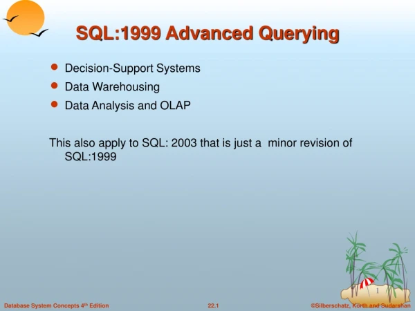
4. Aggregate functions summarize large volumes of data Online Analytical Processing (OLAP) Tools to support interactive analysis of data, allowing data to be summarized and viewed in different ways A histogram partitions the values taken by an attribute into ranges, and computes an aggregate over the values in each range; cumbersome to use standard SQL to construct a histogram. Extension proposed by Red Brick: select percentile, avg (balance) from account group by N_tile (balance, 10) as percentile Data Analysis and OLAP

5. The table above is an example of a cross-tabulation(or cross-tab) also referred to as a pivot-table. In general, a cross-table is a table where values for one attribute form the row headers, values for another attribute form the column headers, and the values in an individual cell are derived as follows. A cross tab with summary rows/columns can be represented by introducing a special value all to represent subtotals. Cross Tabulation of sales by item-name and color

6. Relational Representation of the Data in Figure 22.1

7. Three-Dimensional Data Cube

8. The operation of changing the dimensions used in a cross-tab is called pivoting. An OLAP system provides other functionality as well. For instance, the analyst may wish to see a cross-tab on item-name and color for a fixed value of size, for example, large, instead of the sum across all sizes. Such an operation is referred to as slicing.The operation is sometimes called dicing, particularly when values for multiple dimensions are fixed. The operation of moving from finer-granularity data to a coarser granularity is called a rollup. The opposite operation - that of moving from coarser-granularity data to finer-granularity data – is called a drill down. Online Analytical Processing

9. The earliest OLAP systems used multidimensional arrays in memory to store data cubes, and are referred to as mutidimensional OLAP (MOLAP) systems. Hybrid systems, which store some summaries in memory and store the base data and other summaries in a relational database, are called hybrid OLAP (HOLAP) systems. OLAP Implementation

10. Hierarchies on Dimensions

11. Cross Tabulation of sales With Hierarchy on item-name

12. Data Analysis (Cont.) Total Medium Small Large 8 20 35 10 310 5 Light Dark 53 35 28 45 15 88 Total • Cross-tabulation of number by size and color of sample relation sales with the schema Sales(color, size, number).

13. Can represent subtotals in relational form by using the value all E.g. : obtain (Light, all, 53) and (Dark, all, 35) by aggregating individual tuples with different values for size for each color. Data Analysis (Cont.) Color Size Number Light Light Light Light Dark Dark Dark Dark all all all all 8 35 10 53 20 10 5 35 28 45 15 88 Small Medium Large all Small Medium Large all Small Medium Large all

14. Rollup: Moving from finer-granularity data to a coarser granularity by means of aggregation. Drill down: Moving from coarser-granularity data finer-granularity data. Proposed extensions to SQL, such as the cube operation help to support generation of summary data The following query generates the previous table. selectcolor, size, sum (number) fromsales groupbycolor, size with cube Data Analysis (Cont.)

15. Figure shows the combinations of dimensions size, color, price In general computing cube operation with n groupby columns gives 2nd different groupby combinations. Data Analysis (Cont.)

16. Like knowledge discovery in artificial intelligence data mining discovers statistical rules and patterns it differs from machine learning in that it deals with large volumes of data stored primarily on disk. Knowledge discovered from a database can be represented by a set of rules. e.g.,: “Young women with annual incomes greater than $50,000 are most likely to buy sports cars” Discover rules using one of two models: 1. The user is involved directly in the process of knowledge discovery. 2. The system is responsible for automatically discovering knowledge from the database by detecting patterns and correlation's in the data. Data Mining

17. General form of rules  X antecedent  consequent X is a list of one or more variables with associated ranges. The rule  transactions T, buys (T, bread)  buys(T, milk) states: if there is a tuple (t1, bread) in the relation buys, there must also be a tuple (t1, milk) in the relation buys. Population: Cross-product of the ranges of the variables in the rule. In the above example, the set of all transactions. Support: Measure of what fraction of the population satisfies both the antecedent and the consequent of the rule. e.g., 10% of transactions buy bread and milk. Confidence : Measure of how often the consequent is true when the antecedent is true. e.g., 80% of transactions that buy bread also buy milk Knowledge Representation Using Rules

18. Classification : Finding rules that partition the given data into disjoint groups (classes) that are relevant for making a decision (e.g.,: which of several factors help classify a person’s credit worthiness). Associations: Useful to determine associations between different items (e.g.,: someone who buys bread is quite likely also to buy milk). Sequence correlations: determine correlations between related sequence data. (e.g., : when bond rates go up stock prices go down within two days.) Some Classes of Data-Mining Problems

19. In user-guided data mining, primary responsibility for discovering rules is with the user. User may runs tests on the database to verify or refute a hypothesis. Confidence and support for rules expressing a hypothesis are derived from the database. An iterative process of forming and refining rules is used. Example: Test the hypothesis “People who hold master’s degrees are the most likely to have an excellent credit rating.” If confidence of rule is low, may refine it into the rule:  peopleP, P.degree = MastersandC.income  75, 000  C.credit = excellent Data-visualization though graphical representations like maps, charts, and color-coding, helps detect patterns in data User-Guided Data Mining

20. Classification rules help assign new objects to a set of classes. E.g., given a new automobile insurance applicant, should he or she be classified as low risk, medium risk or high risk? Classification rules for above example could use a variety of knowledge, such as educational level of applicant, salary of applicant, age of applicant, etc. Classification rules can be compactly shown as a Classification tree. Classification Rules

21. Part of Credit Risk Classification Tree

22. Training set: a data sample in which the grouping for each tuple is already known. Top down generation of classification tree. Each internal node of the tree partitions the data into groups based on the attribute. The data at a node is not partitioned further if either all (or most) of the items at the node belong to the same class, or all attributes have been considered. Such a node is a leaf node. Otherwise the data at the node is partitioned further by picking an attribute for partitioning data at the node. Discovery of Classification Rules

23. Consider credit risk example: Suppose degree is chosen to partition the data at the root. Since degree has a small number of possible values, one child is created for each value. At each child node of the root, further classification is done tuple if required. Here, partitions are defined by income. Since income is a continuous attribute, some number of intervals are chosen, and one child created for each interval. Different classification algorithms use different ways of choosing which attribute to partition on at each node, and what the intervals, if any, are. In general, different branches of the tree could grow to different levels. Different nodes at the same level may use difficult partitioning attributes. Discovery of Classification Rules (Cont.)

24. Example:  transactions T, buys (T, bread)  buys (T, milk) In general: notion of transaction , and its intemset, the set of items contained in the transaction General form of rule:  transactions T, c(T, i1) and . . . and c(T, io)  c(T, i0) where c(T, ik) denotes that transaction T contains item ik. Above can be represented as A  b where A = {i1, i2, . . . , in} and b = io. Support of rule = number of transactions whose itemsets contain A  {b} Usually desire rules with strong support, which will involve only items purchased in a significant percentage of the transactions. Discovery of Association Rules

25. Consider all possible sets of relevant items. For each set find its support (i.e. , how many transactions purchase all items in the set). Use sets with sufficiently high support to generate association rules. From set A generate the rules A - {b} b for each b  A. Support of each of the rules is support of A. Confidence of a rule is support of A divided by support of A - {b}. Discovery of Association Rules (Cont.)

26. Few sets: Determine level of support via a single pass. A count is maintained for each set, initially set to 0. When a transaction is fetched, the count is incremented for each set of items which contained in the itemset of the transaction. Sets with a high count at the end of the pass correspond to items with a high degree of association. Many sets: If memory not enough to hold all counts for all sets Use multiple passes, considering only some sets in each pass. Optimization: Once a set is eliminated because it occurs in too small a fraction of the transactions, none of its supersets needs to be considered. Finding Support

27. A data warehouse is a repository of information gathered from multiple sources. Data Warehousing

28. Provides a single consolidated interface to data Data stored for an extended period, providing access to historical data Data/updates are periodically downloaded form online transaction processing (OLTP) systems. Typically, download happens each night. Data may not be completely up-to-date, but is recent enough for analysis. Running large queries at the warehouse ensures that OLTP systems are not affected by the decision-support workload. Data Warehousing (Cont.)

29. When and how to gather data. Source driven: data source initiates data transfer Destination driven: warehouse initiates data transfer What schema to use. Schema integration Cleaning and conversion of incoming data What data to summarize. Raw data may be too large to store on-line Aggregate values (totals/subtotals) often suffice Queries on raw data can often be transformed by query optimizer to use aggregate values How to propagate updates. Date at warehouse is a view on source data Efficient view maintenance techniques required Issues in Building a Warehouse

30. Information retrieval (IR) systems use a simpler data model than database systems, but provide more powerful querying capabilities within the restricted model. Queries attempt to locate documents that are of interest by specifying, for example, sets of keywords. e.g., find documents containing the words “database systems” Information retrieval systems order answers based on their estimated relevance. e.g., user may really only want documents about database systems, but the system may retrieve all documents that mention the phrase database systems”. Documents may be ordered by, for example, how many times the phrase appears in the document. Information Retrieval Systems

31. Combinations of keywords motorcycle and maintenance computer or micro-processor computer but not database Closeness of keyword s in the and case affects ranking. Some systems allow user to specify that the keywords must occur close to each other. Synonyms To retrieve document title motorcycle repair for the query motorcycle and maintenance, need to realize that maintenance and repair are synonyms Similarity based retrieval - retrieve documents similar to a given document. Similarity may be defined based on metrics such as number of common keywords. Queries

32. Information retrieval systems, unlike traditional database systems, handle: Unstructured documents Searching using keywords and relevance ranking Most information retrieval systems do not handle: High update rates Concurrency control Data structured using more complex data models (e.g., relational or object oriented data models) Complex queries written in, e.g., SQL Differences From Database Systems

33. Documents that contain a specified keyword can be located using an inverted index which maps each keyword Ki to the set Si of identifiers of documents that contain Ki . IR systems save space by using index structures that support only approximate retrieval. May result in: false drop - some relevant documents may not be retrieved. false positive - some irrelevant documents may be retrieved. For many applications a good index should not permit any false drops, but may permit a few false positives. Relevant performance metrics: Precision - what percentage of the retrieved documents are relevant to the query. Recall - what percentage of the documents relevant to the query were retrieved. Indexing of Documents

34. and operation: Finds documents that contain all of a set of keywords K1, K2, ..., Kn. Retrieve the corresponding sets of identifiers of documents S1, S2, ... Sn. The intersection, S1S2.....Sn, gives the identifiers of the desired set of documents. or operation: Gives the set of all documents that contain at least one of the keywords K1, K2, …, Kn Found by computing the union, S1S2.....Sn, of the sets. Indexing of Documents (Cont.)

35. not operation: Finds documents that do not contain a specified keyword Ki Let Si be the set of identifiers of documents that contain the keyword Ki. Given a set of document identifies S, eliminate documents that contain the specified keyword Ki by taking the difference S-Si A full-text index uses every work in the document as a keyword. Stop words are very commonly occurring words that are useless as key words, e.g, a, an, the, it etc. These are eliminated from the index. Indexing of Documents (Cont.)

36. Storing related documents together facilitates browsing, where a user can see not only requested document but also related ones. Browsing in a library facilitated by classification system that organizes logically related books together. Browsing

37. A Classification Tree

38. Documents can reside in multiple places in a hierarchy in an information retrieval system, since physical location is not important. Classification hierarchy is thus Directed Acyclic Graph (DAG). Classification DAG

39. A Classification DAG for a library information retrieval system

40. The Archie system automatically follows Gopher links to locate information, and creates a centralized index of information found various sites. Web indexing systems (Web crawlers) follow the hypertext links in documents to find other documents, and build an index on the documents. The indices are often full-text indices, and are stored locally at the indexing system. These systems run a background process to find new sites. obtain updated information from known sites. discard defunct sites. Locating of Information on the Web

41. Web indexing systems permit documents to be located even though they are not registered with any central authority. Drawback: poor precision of recall Full text indexing retrieves unrelated documents that just happen to mention the requested keyword HTML extensions now allow documents to be tagged with keywords to be used by search engines; unfortunately, many documents do not provide such keywords. The extremely large number of documents on the Web often leads to far more results than a human can handle. Alternative approach: a cataloging system for the Web, such as that provide by Yahoo Combinations of catalogs and indexing are quite useful Provided by, e.g., Yahoo (www.yahoo.com). Locating of Information on the Web (Cont.)

42. Classification Tree

43. Data-Warehouse Architecture

44. Star Schema For A Data Warehouse

45. A Classification Hierarchy For A Library System

46. A Classification DAG For A Library Information Retrieval System

47. Online Analytical Processing Data that can be modeled as dimension attributes and measure attributes are called multidimensional data. Given a relation used for data analysis, we can identify some of its attributes as measure attributes, since they measure some value, and can be aggregated upon. For instance, the attribute number of the sales relation is a measure attribute, since it measures the number of units sold. Some of the other attributes of the relation are identified as dimension attributes, since they define the dimensions on which measure attributes, and summaries of measure attributes, are viewed. Data Analysis and OLAP

48. SQL:1999 also supports generalizations of the group by constructs, using the cube and rollup constructs. A representative use of the cube construct is; select item-name, color, size, sum(number)fromsalesgroup by cube(item-name, color, size) This query computes the union of eight different groupings of the sales relation: { (item-name, color, size), (item-name, color), (item-name, size), (color, size), (item-name), (color), (size), ( ) } Where ( ) denotes an empty group by list. For each grouping, the result contains the null value for attributes not present in the grouping. For instance, with occurrences of all replaced by null, can be computed by the query select item-name, color, sum(number)from salesgroup by cube(item-name, color) Extended Aggregation

49. A representative rollup construct is select item-name, color, size, sum(number)from salesgroup by rollup(item-name, color, size) Here only four grouping are generated: { (item-name, color, size), (item-name, color), (item-name), ( ) } Rollup can be used to generate aggregates at multiple levels of ahierarchy on a column. For instance, we have a table itemcategory(item-name, category) giving the category of each item. Then the query select category, item-name, sum(number)from sales, categorywhere sales.item-name = itemcategory.item-namegroup by rollup(category, item-name) would give a hierarchical summary by item-name and by category. Extended Aggregation (Cont.)

50. Multiple rollups and cubes can be used in a single group by clause.For instances, the following query select item-name, color, size, sum(number)from salesgroup by rollup(item-name), rollup(color, size) generates the groupings { (item-name, color, size), (item-name, color), (item-name), (color, size), (color), ( ) } The function grouping can be applied on an attribute; it returns 1 if the value is a null value representing all, and returns 0 in all other cases. Consider the following query: select item-name, color, size, sum(number),grouping(item-name) as item-name-flag,grouping(color) as color-flag,grouping(size) as size-flag,from salesgroup by cube(item-name, color, size) Extended Aggregation (Cont.)