Supply & Demand
Supply & Demand. APEC 3001 Summer 2007 Readings: Chapter 2 in Frank. Objectives. Demand & Supply and Law of Demand & Supply Describing Markets Market Equilibrium & The Function of Price Consumer & Producer Surplus and the Efficiency of Market Equilibrium Equity of Market Equilibrium

Supply & Demand
E N D
Presentation Transcript
Supply & Demand APEC 3001 Summer 2007 Readings: Chapter 2 in Frank
Objectives • Demand & Supply and Law of Demand & Supply • Describing Markets • Market Equilibrium & The Function of Price • Consumer & Producer Surplus and the Efficiency of Market Equilibrium • Equity of Market Equilibrium • Effect of Taxes & Subsidies On Market Equilibrium & Efficiency • Determinants of Supply & Demand and Quantity Supplied & Demanded • Predicting Price & Quantity Changes for Changes in Market Conditions
General Definitions • Product: • A good or service. • Real Price: • The price of a product relative to the price of other products. • Buyer: • A person who wants to purchase a product. • Seller: • A person who wants to sell a product.
Demand & Supply Definitions • Demand (Curve/Function): • The relationship between the price of a product and the quantity buyers want to purchase. • Quantity Demanded: • The amount of product buyers want to purchase at a given price. • Supply (Curve/Function): • The relationship between the price of a product and the quantity sellers want to offer. • Quantity Supplied: • The amount of product sellers want to offer at a given price.
Law of Demand & Supply • Law of Demand: • The observation that when the price of a product falls, people buy more of it. • Law of Supply: • The observation that when the price of a product rises, people sell more of it.
Describing Demand & Supply • Tabular • Graphical • Specific Function • General Linear Function • Really General Function
Tabular Example Supply Demand
Demand Specific QD = 1,000 - 20P P = 50 – 0.05QD General Linear QD = aD - bDP P = aD/bD – QD/ bD Really General QD = D(P) P = D-1(QD) Supply Specific QS = 20P P = 0.05QS General Linear QS = aS + bSP P = aS/bS + QS/bS Really General QS = S(P) P = S-1(QS) Function Examples
Law of Demand Negative Relationship Between Quantity Demanded & Price Demand Downward Sloping bD < 0 D’(P) < 0 D-1’(QD) < 0 Law of Supply Positive Relationship Between Quantity Supplied & Price Supply Upward Sloping bS > 0 S’(P) > 0 S-1’(QS) > 0 Implications of the Law of Supply & Demand
Describing MarketsDefinition • Market: • A collection of buyers and sellers voluntarily exchanging a product. Important: Exchange Is Voluntary
Function Market Example • Specific • QD = 1,000 - 20P • QS = 20P • General Linear • QD = aD - bDP • QS = aS + bSP • Really General • QD = D(P) • QS = S(P)
Market Equilibrium & The Function of PriceDefinitions • Excess Demand/Shortage: • The amount by which the quantity demanded exceeds the quantity supplied at a given price. • Excess Supply/Surplus: • The amount by which the quantity supplied exceeds the quantity demanded at a given price. • Equilibrium Price: • The price at which there is no surplus or shortage. • Equilibrium Quantity: • The quantity at which there is no surplus or shortage.
Graphical Example of Market Equilibrium S P* = $25 Q* = 500 D
Specific Function Example QD* = QS* = Q* for QD* = 1,000 - 20P* & QS* = 20P* 1,000 - 20P* = 20P* 1,000 - 20P* + 20P* = 20P* + 20P* 1,000 = 40P* P* = 25 Q* = QD* = 1,000 – 20 25 = 500 Q* = QS* = 20 25 = 500
General Linear Function Example QD* = QS* = Q* for QD* = aD - bDP* & QS* = aS + bSP* aD - bDP*= aS + bSP* aD - aS - bDP* + bDP*= aS - aS + bSP* + bDP* aD – aS = (bS+bD) P* P* = (aD – aS)/ (bS+bD) Q* = QD* = aD - bD ((aD – aS) / (bS+bD)) = (aDbS + aSbD) / (bS+bD) Q* = QS* = aS + bS ((aD – aS) / (bS+bD)) = (aDbS + aSbD) / (bS+bD)
Really General Function Example QD* = QS* = Q* for QD* = D(P*) & QS* = S(P*) D(P*) = S(P*) With really general function, we cannot solve explicitly for P* and Q*.
How do markets find equilibrium? • Suppose the demand and supply for a Prius is • QD = 1,000 - 20P • QS = 20P • Further suppose the price on the table for a Prius is $15K. • QD = 1,000 – 20 15 = 700 • QS = 20 15 = 300 • QD > QS means there is a shortage, so all interested sellers can make their sales, but all interested buyers will not find an agreeable seller. • If you are a buyer who values a Prius more than $15K, wouldn’t you be willing to offer a price higher than $15K? • As long as there is a shortage, some buyers are willing to pay a higher price in order to make a purchase.
Graphical Example of a Market Shortage P = $15 QD = 700 QS = 300 S 15 D Shortage = 400
How do markets find equilibrium? • Again, suppose the demand and supply for a Prius is • QD = 1,000 - 20P • QS = 20P • Further suppose the price on the table for a Prius is $35K. • QD = 1,000 – 20 35 = 300 • QS = 20 35 = 700 • QS > QD means there is a surplus, so all interest buyers can make a purchase, but all interested sellers cannot find an agreeable buyer. • If you are a seller who values a Prius less than $35K, wouldn’t you be willing to offer a price lower than $35K? • As long as there is a surplus, some sellers are willing to accept a lower price in order to make a sale.
Graphical Example of a Market Surplus P = $15 QD = 300 QS = 700 Surplus = 400 S 35 D
Functions of Price • Rationing Function • directs the existing supply of product to those who value it most. • Allocative Function • directs resources toward the production of product whose price exceeds cost and away from product whose cost exceeds price.
Consumer & Producer Surplus and the Efficiency of Market EquilibriumDefinitions • Efficiency: • People doing the best they can with what they have. • Consumer Surplus: • The dollar amount consumers benefit from purchases. • Producer Surplus: • The dollar amount sellers benefit from sales.
Consumer & Producer Surplus for Individual Trade S 35 Consumer Surplus = $10 Producer Surplus = $10 15 D
Consumer & Producer Surplus for Market Equilibrium Total Surplus (TS) = CS + PS = area abc a Consumer Surplus (CS) = area abd S Producer Surplus (PS) = area bcd Consumer Surplus b d Producer Surplus D c
Consumer & Producer Surplus for Market Surplus a S Surplus CS b g 35 Lost CS Gained PS c f h Lost CS Lost PS PS d D e
Consumer Surplus With Market Equilibrium area acf With Market Surplus area abg Change Loss area bch area bhfg Producer Surplus With Market Equilibrium area cef With Market Surplus area bdeg Change Loss area cdh Gain area bhfg Effect of Market Surplus on Consumer & Producer Surplus
Effect of Market Surplus on Total Surplus • With Market Equilibrium • area ace • With Market Surplus • area abde • Change • Loss • area bcd
Winners & Losers with Market Surplus • Consumers (CS) • Loser (abg < acf) • Producer (PS) • Winner if bhfg > cdh • Loser if bhfg < cdh • Consumers & Producers (TS) • Loser (abde < ace)
Consumer & Producer Surplus for Market Shortage a S Shortage b CS c g h Lost CS Lost PS Gained CS Lost PS f 15 d PS D e
Consumer Surplus With Market Equilibrium area acg With Market Surplus area abdf Change Loss area bch Gain area dfgh Producer Surplus With Market Equilibrium area ceg With Market Surplus area def Change Loss area cdh area dfgh Effect of Market Shortage on Consumer & Producer Surplus
Effect of Market Shortage on Total Surplus • With Market Equilibrium • area ace • With Market Surplus • area abde • Change • Loss • area bcd
Winners & Losers with Market Shortage • Consumers (CS) • Winner if dfgh > bch • Loser if dfgh < bch • Producer (PS) • Loser (def < ceg) • Consumers & Producers (TS) • Loser (abde < ace)
Summary • If the price is above the equilibrium price, a market surplus occurs: • Consumers are worse off. • Producers may be better or worse off. • Even if producers are better off, their gain is less than consumer losses. • Inefficient! • If the price is below the equilibrium price, a market shortage occurs: • Consumers may be better or worse off. • Producers are worse off. • Even if consumers are better off, their gain is less than producer losses. • Inefficient! • Conclusion: • The equilibrium market price results in an efficient allocation of resources.
Equity of Market EquilibriumDefinitions • Equity: • The state of being fair or reasonable. • Price Floor: • Minimum statutory price. • Price Ceiling: • Maximum statutory price.
Are price floors & ceilings equitable? • Price floors create a market surplus: • Consumers are worse off. • Producers may be better or worse off. • If producers are better off & we want them to be better off this outcome may be more equitable. • Price ceilings create a market shortage: • Consumers may be better or worse off. • Producers are worse off. • If consumers are better off & we want them to be better off this outcome may be more equitable. • Conclusion: • Price floors & ceilings may or may not be more equitable. There are no guarantees!
Are price floors & ceilings efficient? • Price floors create a market surplus: • Consumers are worse off. • Producers may be better or worse off. • Even if producers are better off, their gain is less than consumer losses. • Inefficient! • Price ceilings create a market shortage: • Consumers may be better or worse off. • Producers are worse off. • Even if consumers are better off, their gain is less than producer losses. • Inefficient! • Conclusion: • Price floors & ceilings definitely result in an inefficient allocation of resources.
Effect of Taxes & Subsidies On Market Equilibrium & EfficiencyDefinitions • Sales Tax: • Charge to a buyer/seller collected by government for the purchase/sale of a product. • Sales Subsidy: • Payment to a buyer/seller from government for the purchase/sale of a product.
More Definitions • Unit Tax (tU): • A tax per unit purchased/sold. • Unit Subsidy (sU): • A subsidy per unit purchased/sold. • Ad Valorem Tax (tA): • A tax that is proportional to the price of the product purchased/sold. • Ad Valorem Subsidy (sA): • A subsidy that is proportional to the price of the product purchased/sold.
Tax (PS > PD) Unit PS = PD – tU PS + tU = PD Ad Valorem PS = PD(1 - tA) PS / (1 - tA) = PD Subsidy (PS < PD) Unit PS = PD + sU PS - sU = PD Ad Valorem PS = PD(1 + sA) PS / (1 + sA) = PD Price Relationships With Taxes & Subsidies
Graphical Example of Unit Tax (tU = $10K) S(PS) tU = $10 D(PS) tU = $10 D(PS + tU)
Graphical Example of Unit Tax (tU = $10K)Another Perspective D(PD) S(PD - tU) S(PD) tU = $10 tU = $10
Function Examples With Unit Tax (tU) • Specific • QD = 1,000 - 20PD • QS = 20PS • PS + 10 = PD • General Linear • QD = aD - bDPD • QS = aS + bSPS • PS + tU = PD • Really General • QD = D(PD) • QS = S(PS) • PS + tU = PD
Tabular Example of Market Equilibrium WithUnit Tax (tU = $10K)
Graphical Example of Market Equilibrium WithUnit Tax (tU = $10K) PS* = 20 PD* = 30 Q* = 400 S(PS) D(PS) D(PS + tU)
Graphical Example of Market Equilibrium WithUnit Tax (tU = $10K) Another Perspective PS* = 20 PD* = 30 Q* = 400 S(PD - tU) D(PD) S(PD)