SQL Server Parallel Data Warehouse: Supporting Large Scale Analytics
SQL Server Parallel Data Warehouse: Supporting Large Scale Analytics. José Blakeley, Software Architect Database Systems Group, Microsoft Corporation. SQL Server PDW Overview. Workload Types. Online Transaction Processing (OLTP) Balanced read-update ratio (60%-40%)

SQL Server Parallel Data Warehouse: Supporting Large Scale Analytics
E N D
Presentation Transcript
SQL Server Parallel Data Warehouse:Supporting Large Scale Analytics José Blakeley, Software Architect Database Systems Group, Microsoft Corporation
SQL Server PDW Overview JHU DIR March 2011
Workload Types • Online Transaction Processing (OLTP) • Balanced read-update ratio (60%-40%) • Fine-grained inserts and updates • High transaction throughput e.g., 10s K/s • Usually very short transactions e.g., 1-3 tables • Sometimes multi-step e.g., financial • Relatively small data sizes e.g., few TBs • Data Warehousing and Business Analysis (DW) • Read-mostly (90%-10%) • Few updates in place, high-volume bulk inserts • Concurrent query throughput e.g., 10s K / hr • Per query response time < 2 s • Snowflake, star schemas are common e.g., 5-10 tables • Complex queries (filter, join, group-by, aggregation) • Very large data sizes e.g., 10s TB - PB Day-to-day business Analysis over historical data JHU DIR March 2011
SQL Server Parallel Data Warehouse • Shared-nothing, distributed, parallel DBMS • Built-in data and query partitioning • Provides single system view over a cluster of SQL Servers • Appliance concept • Software + hardware solution • Choice of hardware vendors (e.g., HP, Dell, NEC) • Optimized for DW workloads • Bulk loads (1.2 – 2.0 TB/hr) • Sequential scans (700 TB in 3hr) • Scale from 10 Terabytes to Petabytes • 1 rack manages ~40 TB • 1 PB will need ~25 racks JHU DIR March 2011
Hardware Architecture Compute Nodes Storage Nodes SQL SQL SQL SQL SQL SQL SQL SQL SQL Control Nodes Active / Passive Client Drivers (ODBC, OLE-DB, ADO.NET) Management Servers Data Center Monitoring Dual Infiniband Dual Fiber Channel Landing Zone ETL Load Interface Backup Nodes Spare Compute Node Corporate Backup Solution 2 Rack Appliance JHU DIR March 2011
Software Architecture Internet Explorer Query Tool MS BI (AS, RS) DWSQL 3rd Party Tools IIS Data Access (OLEDB, ODBC, ADO.NET, JDBC) Admin Console Compute Node Compute Nodes Data Movement Service Compute Nodes PDW Engine Data Movement Service SQL Server User Data Landing Zone Node SQL Server Data Movement Service DW Authentication DW Configuration DW Schema TempDB Control Node JHU DIR March 2011
Key Software Functionality • PDW Engine • Provides single system image • SQL compilation • Global metadata and appliance configuration • Global query optimization and plan generation • Global query execution coordination • Global transaction coordination • Authentication and authorization • Supportability (HW and SW status info via DMVs) • Data Movement Service • Data movement across the appliance • Distributed query execution operators • Parallel Loader • Runs from the Landing Zone • SSIS or command line tool • Parallel Database Copy • High performance data export • Enables Hub-Spoke scenarios • Parallel Backup/Restore • Backup files stored on Backup Nodes • Backup files may be archived into external device/system JHU DIR March 2011
Query Processing • SQL statement compilation • Parsing, validation, optimization • Builds an MPP execution plan • A sequence of discrete parallel QE “steps” • Steps involve SQL queries to be executed by SQL Server at each compute node • As well as data movement steps • Executes the plan • Coordinates workflow among steps • Assembles the result set • Returns result set to client JHU DIR March 2011
18,000,048,306 rows Example DW Schema 4,500,000,000 rows SELECTTOP10 L_ORDERKEY, SUM(L_EXTENDEDPRICE*(1-L_DISCOUNT)) AS REVENUE, O_ORDERDATE, O_SHIPPRIORITY FROMCUSTOMER, ORDERS, LINEITEM WHEREC_MKTSEGMENT= 'BUILDING' AND C_CUSTKEY = O_CUSTKEY AND L_ORDERKEY = O_ORDERKEY AND O_ORDERDATE < ‘2010-03-05' AND L_SHIPDATE > ‘2010-03-05' GROUPBYL_ORDERKEY, O_ORDERDATE, O_SHIPPRIORITY ORDERBYREVENUE DESC, O_ORDERDATE 30,000,000 rows 600,000,000 rows 2,400,000,000 rows 25 rows 5 rows JHU DIR March 2011 450,000,000 rows 9/19/2014
Example – Schema TPCH ---------------------------------------------------------------------- -- Customer Table -- distributed on c_custkey ---------------------------------------------------------------------- CREATE TABLE customer ( c_custkeybigint, c_namevarchar(25), c_addressvarchar(40), c_nationkey integer, c_phone char(15), c_acctbal decimal(15,2), c_mktsegment char(10), c_commentvarchar(117)) WITH (distribution=hash(c_custkey)) ; ---------------------------------------------------------------------- -- Orders Table ---------------------------------------------------------------------- CREATE TABLE orders ( o_orderkeybigint, o_custkeybigint, o_orderstatus char(1), o_totalprice decimal(15,2), o_orderdate date, o_orderpriority char(15), o_clerk char(15), o_shippriority integer, o_commentvarchar(79)) WITH (distribution=hash(o_orderkey)) ; ---------------------------------------------------------------------- -- LineItem Table -- distributed on l_orderkey ---------------------------------------------------------------------- CREATE TABLE lineitem ( l_orderkeybigint, l_partkeybigint, l_suppkeybigint, l_linenumberbigint, l_quantity decimal(15,2), l_extendedprice decimal(15,2), l_discount decimal(15,2), l_tax decimal(15,2), l_returnflag char(1), l_linestatus char(1), l_shipdate date, l_commitdate date, l_receiptdate date, l_shipinstruct char(25), l_shipmode char(10), l_commentvarchar(44)) WITH (distribution=hash(l_orderkey)) ; JHU DIR March 2011
Example - Query Ten largest “building” orders shipped since March 5, 2010 SELECTTOP10 L_ORDERKEY, SUM(L_EXTENDEDPRICE*(1-L_DISCOUNT)) AS REVENUE, O_ORDERDATE, O_SHIPPRIORITY FROMCUSTOMER, ORDERS, LINEITEM WHEREC_MKTSEGMENT= 'BUILDING' AND C_CUSTKEY = O_CUSTKEY AND L_ORDERKEY = O_ORDERKEY AND O_ORDERDATE < ‘2010-03-05' AND L_SHIPDATE > ‘2010-03-05' GROUPBYL_ORDERKEY, O_ORDERDATE, O_SHIPPRIORITY ORDERBYREVENUE DESC, O_ORDERDATE JHU DIR March 2011
Example – Execution Plan ------------------------------ -- Step 1: create temp table at control node ------------------------------ CREATE TABLE [tempdb].[dbo].[Q_[TEMP_ID_664]] ( [l_orderkey] BIGINT, [REVENUE] DECIMAL(38, 4), [o_orderdate] DATE, [o_shippriority] INTEGER ); ------------------------------ -- Step 2: create temp tables at all compute nodes ------------------------------ CREATE TABLE [tempdb].[dbo].[Q_[TEMP_ID_665]_[PARTITION_ID]] ( [l_orderkey] BIGINT, [l_extendedprice] DECIMAL(15, 2), [l_discount] DECIMAL(15, 2), [o_orderdate] DATE, [o_shippriority] INTEGER, [o_custkey] BIGINT, [o_orderkey] BIGINT ) WITH ( DISTRIBUTION = HASH([o_custkey]) ); ------------------------------- -- Step 3: SHUFFLE_MOVE -------------------------------- SELECT [l_orderkey], [l_extendedprice], [l_discount], [o_orderdate], [o_shippriority], [o_custkey], [o_orderkey] FROM [dwsys].[dbo].[orders] JOIN [dwsys].[dbo].[lineitem] ON ([l_orderkey] = [o_orderkey]) WHERE ([o_orderdate] < ‘2010-03-05' AND [o_orderdate] >= ‘2010-09-15 00:00:00.000') INTO Q_[TEMP_ID_665]_[PARTITION_ID] SHUFFLE ON (o_custkey); ------------------------------ -- Step 4: PARTITION_MOVE ------------------------------ SELECT [l_orderkey], sum(([l_extendedprice] * (1 - [l_discount]))) AS REVENUE, [o_orderdate], [o_shippriority] FROM [dwsys].[dbo].[customer] JOINtempdb.Q_[TEMP_ID_665]_[PARTITION_ID] ON ([c_custkey] = [o_custkey]) WHERE [c_mktsegment] = 'BUILDING' GROUP BY [l_orderkey], [o_orderdate], [o_shippriority] INTO Q_[TEMP_ID_664]; ------------------------------ -- Step 5: Drop temp tables at all compute nodes ------------------------------ DROP TABLE tempdb.Q_[TEMP_ID_665]_[PARTITION_ID]; ------------------------------- -- Step 6: RETURN result to client -------------------------------- SELECT TOP 10 [l_orderkey], sum([REVENUE]) AS REVENUE, [o_orderdate], [o_shippriority] FROMtempdb.Q_[TEMP_ID_664] GROUP BY [l_orderkey], [o_orderdate], [o_shippriority] ORDER BY [REVENUE] DESC, [o_orderdate] ; ------------------------------- -- Step 7: Drop temp table at control node -------------------------------- DROP TABLE tempdb.Q_[TEMP_ID_664]; JHU DIR March 2011
Microsoft Column-store Technology VertiPaq and VertiScan In-memory BI (IMBI) Slides by Amir Netz JHU DIR March 2011
In-Memory BI Technology • Developed by SQL Analysis Services (OLAP) team • Column-based storage and processing • Only touch the columns needed for the query • Compression (VertiPaq) • Columnar data is more compressible than row data • Fast in-memory processing (VertiScan) • Filter, grouping, aggregation, sorting JHU DIR March 2011
How VertiPaq Compression Works Read Raw Data Organize by Columns Phase I: Encoding Dictionary Encoding Value Encoding Convert to uniform representation (Integer Vectors) Encoding is per column 2x – 10x size reduction 1x – 2x size reduction VertiPaqCompression Compression Analysis Hybrid RLE Phase II: Compression Minimize storage space Compression is per 8M row segments 75%-95% of data 5%-25% of data Run Length Encoding (RLE) Bit Packing JHU DIR March 2011 ~100x size reduction 2x – 4x size reduction
436,892,631 rows APPX – 1TB 41 rows 34 rows Star Join Schema SELECTFE0.RegionName, FL0.FiscalYearName, SUM (A.ActualRevenueAmt) FROMTECSPURSL00 A JOINSalesDate L ONA.SalesDateID = L.SalesDateID JOINUpperGeography UG ONA.TRCreditedSubsidiaryId = UG.CreditedSubsidiaryID JOINRegion FE0 ONUG.CreditedRegionID = FE0.RegionID JOINFiscalYear FL0 ONL.FiscalYearID = FL0.FiscalYearID GROUP BY FE0.RegionName, FL0.FiscalYearName 118 rows 13,517 rows JHU DIR March 2011 9/19/2014
Column-Store on APPX • Response time < 2s common • Smaller variance in response time more predictable query performance JHU DIR March 2011
THANKS! JHU DIR March 2011