Chapter 14 Randomized algorithms
Chapter 14 Randomized algorithms. Introduction Las Vegas and Monte Carlo algorithms Randomized Quicksort Randomized selection Testing String Equality Pattern Matching Random Sampling Primality Testing. 14.1 Introduction. Definition:

Chapter 14 Randomized algorithms
E N D
Presentation Transcript
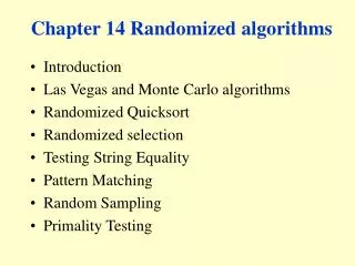
Chapter 14 Randomized algorithms • Introduction • Las Vegas and Monte Carlo algorithms • Randomized Quicksort • Randomized selection • Testing String Equality • Pattern Matching • Random Sampling • Primality Testing
14.1 Introduction • Definition: A Randomized algorithm can be defined as one that receives, in addition to its input, a stream of random bits that it can use in the course of its action for the purpose of making random choices.
14.1 Introduction • Advantages: • Often the execution time or space requirement of a randomized algorithm is smaller than that of the best deterministic algorithm that we know of for the same problem. • If we look at the various randomized algorithms that have been invented so far, we find that invariably they are extremely simple to comprehend and implement.
14.1 Example 14.1 Suppose we have a polynomial expression in n variables, say f(x1, x2, …, xn), and we wish to check whether or not f is identically zero. To do this analytically could be a horrendous job. Suppose, instead, we generate a random n vector (r1, r2, …, rn) of real numbers and evaluate f(r1, r2, …, rn). If we know that . If f(r1, r2, …, rn) = 0, then either f is identically zero or we have been extremely lucky in our choice of (r1, r2, …, rn). If we repeat this several times and keep on getting f = 0, then we conclude that f is identically zero. The probability that we have made an error is negligible.
14.2 Las Vegas and Monte Carlo Algorithms • Classify: Randomized algorithms can be classified into two categories: • Las Vegas algorithms: It constitutes those randomized algorithms that always give a correct answer, or do not give an answer at all. • Monte Carlo Algorithms: always gives an answer, but may occasionally produce an answer that is incorrect. However, the probability of producing an incorrect answer can be made arbitrarily small by running the algorithm repeatedly with independent random choices in each run.
14.3 Randomized Quicksort • Randomized Quicksort is one of the most popular randomized algorithms. • The original Quicksort requires that all permutations of the input elements are equally likely. • Randomized Quicksort selects the pivot on which to split the elements randomly. The result of choosing the pivot randomly is to relax the assumption that all permutations of the input elements are equally likely. • The algorithm’s expected running time is (nlogn).
14.3 Algorithm 14.1 RandomizedQuickSort Input: An array A[1..n] of n elements. Output: The elements in A sorted in non-decreasing order. 1. rquicksort(1, n) Procedure:rquicksort(low, high) 1. iflow < highthen • v random(low, high) • Interchange A(low) and A(v) • SPLIT(A[low, high], w) //w is the new position of the pivot • rquicksort(low, w - 1) • rquicksort(w + 1, high) 7. end if
14.4 Randomized Selection • Consider algorithm SELECT, which was presented Sec. 6.5. We have shown that the algorithm’s running time is (n) with a large multiplicative constant that makes the algorithm impractical, especially for small and moderate values of n. In this section, we present a randomized Las Vegas algorithm for selection that is both simple and fast. Its expected running time is (n) with a small multiplicative constant, and (n2) in the worst case.
14.4 Algorithm 14.2 RandomizedSelect Input: An array A[1..n] of n elements and an integer k, Output: The kth smallest element in A. 1. rselect(A, 1, n, k) Procedure:rselect(A, low, high, k) 1. v random(low, high) 2. x A[v] 3. Partition A[low..high] into three arrays: A1 = {a | a < x} A2= {a | a = x} A3= {a | a > x} 4. case |A1| >= k: returnrselect(A1, 1, |A1|, k) |A1| + |A2| >= k: returnx |A1| + |A2| < k: returnrselect(A3, 1, |A3|, k - |A1| - |A2|) 5. end case
14.4 Theorem 14.1 The expected number of element comparisons performed by Algorithm RandomizedSelect on input of size n is less than 4n. Its expected running time is .
14.5 Testing String Equality • Problem: Suppose that two parties A and B can communicate over a communication channel, which we will assume to be very reliable. A has a very long string x and B has a very long string y, and they want to determine whether x=y.
14.5 Testing String Equality • solution: Let A to derive from x a much shorter string that could serve as a “fingerprint” of x and send it to B. B then would use the same derivation to obtain a fingerprint for y, and then compare the two fingerprint. If they are equal, then B would assume that x=y; otherwise he would conclude that x/=y. B then notifies A of the outcome of the test.
14.5 Testing String Equality • Fingerprinting: For a string w, let I(w) be the integer represented by the bit string w. To choose a prime number p and then use the fingerprint function: Ip(x)=I(x)(mod p) If p is not too large, then the fingerprint Ip(x) can be sent as a short string. The number of bits to be transmitted is thus O(logp). If Ip(x)/= Ip(y), then obviously x/=y. However, the converse is not true. That is, if If Ip(x)= Ip(y), then it is not necessarily the case that x=y. We refer to this phenomenon as a false match. A false match occurs if x/=y, but If Ip(x)= Ip(y), i.e., p divides I(x)-I(y).
14.5 Algorithm 14.3 StringEqualityTest 1.A chooses p at random from the set of primes less than M. 2. A sends p and Ip(x) to B. 3. B checks whether Ip(x) = Ip(y) and confirm the equality or inequality of the two stings x and y.
14.5 Example 14.2 Suppose that x and y are one million bits each, i.e., n=1,000,000. Then M=2×1012=240.8631. In this case, the number of bits required to transmit p is at most [log M]+1=40+1=41. The number of bits required to transmit the fingerprint of x is at most [log(p-1)]+1≤[logM]+1=41. Thus, the total number of bits transmitted is at most 82. The probability of failure in one transmission is at most 1/n=1/1,000,000. Since [log logn]=5, repeating the algorithm five times reduces the probability of false match to n-[log logn]=(106)-5=10-30, which is negligible.
14.6 Pattern Matching • Problem: Given a string of text X=x1x2…xn and a pattern Y=y1y2…ym, where m<=n, determine whether or not the pattern appears in the text. Assume that the text alphabet is ={0, 1}.
14.6 Pattern Matching • Solution: Instead of comparing the pattern with each block X(j)=xjxj+1…xj+m-1, we will compare the fingerprint Ip(Y) of the pattern with the fingerprints Ip(X(j)) of the blocks of text. The fingerprints of the new block X(j+1) can easily be computed from the fingerprints of X(j): Let Wp=2m(mod p), then
14.6 Algorithm 14.4 PatternMatching Input: A string of text X and a pattern Y of length n and m, respectively. Output: The first position of Y in X if Y occurs in X; otherwise 0. 1. Choose p at random from the set of primes less than M. 2. j 1 3. Compute Wp=2m(mod p), Ip(Y) and Ip(Xj) 4. whilej≤n-m+1 • ifIp(Xj)=Ip(Y)then return j //A match is found(probaly) • Compute Ip(Xj) using Ip(X(j+1))=(2Ip(X(j))-Wpxj+xj+m) (mod p) • j j+1 8. end while 9. return 0 //Y does not occur in X(definitely)
14.6 Pattern Matching • Time complexity: • By brute-force method: O(mn) • By randomized method: O(m+n) • The probability of a false match: 1/n • To convert the algorithm into a Las Vegas algorithm: Whenever the two fingerprints Ip(Y) and Ip(X(j)) match, the two strings are tested for equality. The expected time complexity of this Las Vegas algorithm becomes O(n+m)(1-1/n)+mn(1/n)=O(n+m).
14.7 Random Sampling • Problem: To select a sample of m elements randomly from a set of n elements, where m<n. • Solution: First mark all the n elements as unselected. Next, repeat the following step until exactly m elements have been selected. • The time complexity: (n).
14.7 Algorithm14.5 RandomSampling Input: Two positive integers m, n with m<n. Output: An array A[1..n] of m distinct positive integers selected randomly from the set {1, 2, … , 3} 1. comment: S[1..n] is a boolean array indicating whether an integer has been selected. 2. for i 1 to n 3. S[i] false 4. end for 5. k 0 6. whilek<m 7. r random(1, n) 8. if notS[r] then 9. k k+1 10. A[k] r 11. S[r] true 12. end if 13. end while
14.8 Primality Testing • Problem: To test whether a given positive integer n is prime. It is a well-know Monte Carlo algorithm. • Solution: • The obvious method of repeatedly dividing by the numbers from 2 to . • To proof that a number is composite. • Base on Fermat’s theorem.
14.8 Algorithm14.6 Expmod Input: positive integers a, m and n with m≤n. Output: am (mod n). 1. Let the binary digits of m be bk, bk-1, … , b0. 2. c 1 3. for j k down to 0 4. c c2 (mod n) 5. ifbj=1 then c ac (mod n) 6. end for 7. returnc
14.8 Theorem 14.2 (Fermat’s Theorem) If n is prime, then for all a≠0 (mod n) we have an-1 ≡1 (mod n)
14.8 Algorithm 14.7 PTEST1 Input: A positive odd integer n≥5. Output: prime if n is prime; otherwise composite. 1. if Expmod(2, n-1, n) ≡1 (mod n) then return prime //probably 2. else return composite //definitely
14.8 Algorithm 14.8 PTEST2 Input: A positive odd integer n≥5. Output: prime if n is prime; otherwise composite. 1. a random(2, n-2) 2. if Expmod(2, n-1, n) ≡1 (mod n) then return prime //probably 2. else return composite //definitely
14.8 Lemma 14.1 If n is not a Carmichael number, then Algorithm PTEST2 will detect the compositeness of n with probability at least ½.
14.8 Algorithm 14.9 PTEST3 Input: A positive odd integer n≥5. Output:prime if n is prime; otherwise composite. 1. q 0; m n-1 2. repeat //find q and m 3. m m/2 4. q q+1 5. untilm is odd 6. a random(2, n-2) 7. x Expmod(a, m, n) 8. if x=1 then return prime //probably 9. for j 0 to q-1 10. ifx ≡ 1 (mod n) then return prime //probably 11. x x2 (mod n) 12. end for 13. return composite //definitely
14.8 Theorem 14.3 If Algorithm PTEST3 returns “composite”, then n is composite.
14.8 Algorithm 14.10 PrimalityTest Input: A positive odd integer n≥5. Output:prime if n is prime; otherwise composite. 1. q 0; m n-1; k [logn] 2. repeat //find q and m 3. m m/2 4. q q+1 5. untilm is odd 6. fori 1 to k 7. a random(2, n-2) 8. x Expmod(a, m, n) 9. ifx = 1 then returnprime //probably 10. forj 0 to q-1 11. ifx≡ -1 (mod n) then returnprime //probably 12. x x2 (mod n) 13. end for 14. end for 15. return composite //definitely
14.8 Theorem 14.4 In tine O(log4n), Algorithm PrimalityTest behaves as follows when presented with an odd integer n≥5: 1. If n is prime, then it outputs prime. 2. If n is composite, then it outputs composite with probably at least 1-1/n.

