Download

1 / 26
260 likes | 291 Views
Understand factor theorem, rational zeros test, Descartes' rule, & multiple zero properties. Learn to factor higher degree polynomials & solve equations. Examples & solutions included.

E N D
Chapter 4 More Nonlinear Functions and Equations Book cover will go here
Real Zeros of Polynomial Functions 4.4 Understand the factor theorem Factor higher degree polynomials Analyze polynomials having multiple zeros Solve higher degree polynomial equations Understand the rational zeros test, Descartes’ rule of signs, and the intermediate value property
Factor Theorem A polynomial f(x) has a factor x – k if and only if f(k) = 0.
Use the graph and the factor theorem to list the factors of f(x). Example: Applying the factor theorem • Solution • The zeros or x-intercepts of f are 2, 1 and 3. Since f(2) = 0, thefactor theorem states that(x + 2) is a factor, and f(1) = 0 implies that • (x 1) is afactor and f(3) = 0 implies (x 3) is a factor. Thus the factors are (x + 2),(x 1), and (x 3).
Zeros with Multiplicity The polynomial f(x) = x2 + 4x + 4 can be written as f(x) = (x+ 2)2. Since the factor (x + 2) occurs twice in f(x), the zero –2 is called azero of multiplicity 2. • The polynomialg(x)= (x+ 1)3(x– 2) has zeros –1 and 2 withmultiplicities3 and 1, respectively: x-intercepts coincide with zeros of g.
Complete Factored Form Suppose a polynomial f(x) = anxn+ … + a2x2 + a1x + a0 has n real zeros c1, c2, c3, …, cn, where a distinct zero is listed as many times as its multiplicity. Then f(x) can be written in complete factored form as f(x) = an(x – c1)(x – c2)(x – c3) …(x – cn)
Write the complete factorization for the polynomial 7x3 – 21x2 – 7x + 21 with given zeros –1, 1 and 3. Solution Leading coefficient is 7. Zeros are –1, 1 and 3 The complete factorization: f(x) = 7(x + 1)(x – 1)(x – 3). Example: Finding a complete factorization
Use the graph of f to factorf(x) = 2x3 – 4x2 – 10x + 12. Example: Factoring a polynomial graphically • Solution • Leading coefficient is 2 • Zeros are –2, 1 and 3 • The complete factorization: • f(x) = 2(x + 2)(x – 1)(x – 3).
The polynomial f(x) = 2x3 2x2 34x – 30 has a zero of –1. Express f(x) in complete factored form. Solution If –1 is a zero, by the factor theorem x + 1 is a factor. Use synthetic division. Example: Factoring a polynomial symbolically
Graphs and Multiple Zeros The polynomial f(x) = 0.02(x + 3)3(x – 3)2has zeros –3 and 3 with multiplicities 3and 2, respectively. At the zero of even • multiplicity the graph does not cross the x-axis (3, 0), whereas the graph does cross thex-axis at the zero of odd multiplicity(–3, 0).
Rational Zeros Test Let f(x) = anxn+ … + a2x2 + a1x + a0,where a ≠ 0, represent a polynomial function f with integer coefficients. If p/q is a rational number written in lowest terms and if p/q is a zero of f, then p is a factor of the constant term and q is a factor of the leading coefficient an.
Find all rational zeros of f(x) = 6x3 5x2 7x + 4 and factor f(x). Solution p is a factor of 4, q is a factor of 6 Any rational zero must occur in the list Example: Finding rational zeros of a polynomial
Evaluate f(x) at each value in the list. Example: Finding rational zeros of a polynomial
There are three rational zeros: –1, Since a third degree polynomial has at most three zeros, the complete factored form is which can written Example: Finding rational zeros of a polynomial
Descartes’ Rule of Signs Let P(x) define a polynomial function with real coefficients and a nonzero constant term, with terms in descending powers of x. • (a)The number of positive real zeros either equals the number of variations in signoccurring in the coefficients of P(x) or is less than the number of variations by apositive even integer.
Descartes’ Rule of Signs Let P(x) define a polynomial function with real coefficients and a nonzero constantterm, with terms in descending powers of x. • (b)The number of negative real zeros either equals the number of variations in signoccurring in the coefficients of P(–x) or is less than the number of variations bya positive even integer.
Determine the possible numbers of positive real zeros and negative real zeros ofP(x) = x4 6x3 + 8x2 + 2x – 1. Solution P(x) has three variations in sign +x4 6x3 + 8x2 + 2x – 1 P(x) has 3, or ( 3 – 2 =) 1 positive real roots Example: Applying Descartes’ rule of signs
P(–x)= (–x)4 6(–x)3 + 8(–x)2 + 2(–x) – 1 = x4 + 6x3 + 8x2 – 2x – 1 P(–x)has one variation in sign, P(x) has only one negative real root. Example: Applying Descartes’ rule of signs
Polynomial Equations Factoring can be used to solve polynomial equations with degree greater than 2. We can also solve the graphically.
Find all real solutions to each equation symbolically. a. 4x4 – 5x2 – 9 = 0 b. 2x3 + 12 = 3x2 + 8x Solution Example: Solving a polynomial equation
The only real solutions are Example: Solving a polynomial equation
b. The solutions are –2, , and 2. Example: Solving a polynomial equation
Solve the equation x3 – 2x – 4 = 0 graphically. Round any solutions to the nearest hundredth. Solution Example: Finding the solution graphically Since there is only one x-intercept the equation has one real solution: x 2.65
Intermediate Value Theorem Let (x1, y1) and (x2, y2) with y1 ≠ y2 and x1 < x2, be two points on the graph of a continuous function f. Then, on the interval x1 ≤ x ≤ x2, f assumes every value between y1and y2at least once.
Applications: Intermediate Value Property There are many examples of the intermediate value property. Physical motion is usually considered to be continuous. Suppose at one time a car is traveling at 20 miles per hour and at another time it is traveling at 40 miles per hour. It is logical to assume that the car traveled 30 miles per hour at least once between these times. In fact, by the inter- mediate value property, the car must have assumed all speeds between 20 and 40 miles per hour at least once.
Divide 6x3 – 3x2+ 2 by 2x2. Solution Example: Dividing by a monomial