Download
1 / 105
1.05k likes | 1.23k Views
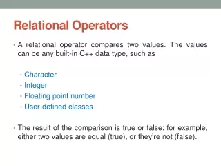
Implementation of Relational Operators. Steps of processing a high-level query. Database. Statistics. Cost Model. Query Optimizer. Query Evaluator. Parsed Query. QEP. Parser. High Level Query. Query Result. Relational Operations. We will consider how to implement:

E N D
Steps of processing a high-level query Database Statistics Cost Model Query Optimizer Query Evaluator Parsed Query QEP Parser High Level Query Query Result
Relational Operations • We will consider how to implement: • Selection () Selects a subset of rows from relation. • Projection ( ) Deletes unwanted columns from relation. • Join ( ) Allows us to combine two relations. • Set-difference ( - ) Tuples in reln. 1, but not in reln. 2. • Union ( U ) Tuples in reln. 1 and in reln. 2. • Aggregation (SUM, MIN, etc.) and GROUP BY
Paradigm • Iteration • Index • B+-tree, Hash • assume index entries to be (rid,pointer) pair • Clustered, Unclustered • Sort • Hash
Schema for Examples Sailors (sid: integer, sname: string, rating: integer, age: real) Reserves (sid: integer, bid: integer, day: dates, rname: string) • Reserves (R): • pR tuples per page, M pages. pR = 100. M = 1000. • Sailors (S): • pS tuples per page, N pages. pS = 80. N = 500. • Cost metric: # of I/Os (pages) • We will ignore output costs in the following discussion.
Equality Joins With One Join Column SELECT * FROM Reserves R, Sailors S WHERE R.sid=S.sid • In algebra: R S. • Most frequently used operation; very costly operation. • join_selectivity = join_size/(#R tuples #S tuples)
Simple Nested Loops Join foreach tuple r in R do foreach tuple s in S do if r.sid == s.sid then add <r, s> to result • For each tuple in the outer relation R, we scan the entire inner relation S. • I/O Cost? • Memory?
Simple Nested Loops Join foreach tuple r in R do foreach tuple s in S do if r.sid == s.sid then add <r, s> to result • For each tuple in the outer relation R, we scan the entire inner relation S. • Cost: M + pR * M * N = 1000 + 100*1000*500 I/Os.
Simple Nested Loops Join foreach tuple r in R do foreach tuple s in S do if r.sid == s.sid then add <r, s> to result • For each tuple in the outer relation R, we scan the entire inner relation S. • Cost: M + pR * M * N = 1000 + 100*1000*500 I/Os. • Memory: 3 pages!
. . . Block Nested Loops Join • Use one page as an input buffer for scanning the inner S, one page as the output buffer, and use all remaining pages to hold ``block’’ of outer R. • For each matching tuple r in R-block, s in S-page, add <r, s> to result. Then read next R-block, scan S, etc. Join Result R & S Hash table for block of R (k < B-1 pages) . . . . . . Output buffer Input buffer for S
Examples of Block Nested Loops • Cost: Scan of outer + #outer blocks * scan of inner • #outer blocks ?
Examples of Block Nested Loops • Cost: Scan of outer + #outer blocks * scan of inner • #outer blocks = no. of pages in outer relation / block size
Examples of Block Nested Loops • Cost: Scan of outer + #outer blocks * scan of inner • #outer blocks = no. of pages in outer relation / block size • With R as outer, block size of 100 pages: • Cost of scanning R is 1000 I/Os; a total of 10 blocks. • Per block of R, we scan S; 10*500 I/Os. • If block size for just 90 pages of R, scan S 12 times.
Examples of Block Nested Loops • Cost: Scan of outer + #outer blocks * scan of inner • #outer blocks = no. of pages in outer relation / block size • With R as outer, block size of 100 pages: • Cost of scanning R is 1000 I/Os; a total of 10 blocks. • Per block of R, we scan S; 10*500 I/Os. • If block size for just 90 pages of R, scan S 12 times. • With 100-page block of S as outer?
Examples of Block Nested Loops • Cost: Scan of outer + #outer blocks * scan of inner • #outer blocks = no. of pages in outer relation / block size • With R as outer, block size of 100 pages: • Cost of scanning R is 1000 I/Os; a total of 10 blocks. • Per block of R, we scan S; 10*500 I/Os. • If block size for just 90 pages of R, scan S 12 times. • With 100-page block of S as outer: • Cost of scanning S is 500 I/Os; a total of 5 blocks. • Per block of S, we scan R; 5*1000 I/Os.
Index Nested Loops Join foreach tuple r in R do search index of S on sid using Ssearch-key = r.sid for each matching key retrieve s; add <r, s> to result • If there is an index on the join column of one relation (say S), can make it the inner and exploit the index. • Cost: M + ( (M*pR) * cost of finding matching S tuples) • For each R tuple, cost of probing S index is about 1.2 for hash index, 2-4 for B+ tree. Cost of then finding S tuples (assuming leaf data entries are pointers) depends on clustering. • Clustered index: 1 I/O (typical), unclustered: upto 1 I/O per matching S tuple.
Examples of Index Nested Loops • Hash-index on sid of S (as inner): • Scan R: 1000 page I/Os, 100*1000 tuples. • For each R tuple: 1.2 I/Os to get data entry in index, plus 1 I/O to get (the exactly one) matching S tuple. Total: 220,000 I/Os. • Hash-index on sid of R (as inner)?
Examples of Index Nested Loops • Hash-index on sid of S (as inner): • Scan R: 1000 page I/Os, 100*1000 tuples. • For each R tuple: 1.2 I/Os to get data entry in index, plus 1 I/O to get (the exactly one) matching S tuple. Total: 220,000 I/Os. • Hash-index on sid of R (as inner): • Scan S: 500 page I/Os, 80*500 tuples. • For each S tuple: 1.2 I/Os to find index page with data entries, plus cost of retrieving matching R tuples. • Assuming uniform distribution, 2.5 reservations per sailor (100,000 / 40,000). Cost of retrieving them is 1 or 2.5 I/Os depending on whether the index is clustered.
Sort-Merge Join • Sort R and S on the join column, then scan them to do a ``merge’’ (on join col.), and output result tuples. • Advance scan of R until current R-tuple >= current S tuple, then advance scan of S until current S-tuple >= current R tuple; do this until current R tuple = current S tuple. • At this point, all R tuples with same value in Ri (current R group) and all S tuples with same value in Sj (current S group) match; output <r, s> for all pairs of such tuples. • Then resume scanning R and S. • R is scanned once; each S group is scanned once per matching R tuple. (Multiple scans of an S group are likely to find needed pages in buffer.)
Example of Sort-Merge Join • Cost?
Example of Sort-Merge Join • Cost: 2M*K1+ 2N*K2+ (M+N) • K1 and K2 are the number of passes to sort R and S respectively • The cost of scanning, M+N, could be M*N (very unlikely!)
Example of Sort-Merge Join • Cost: 2M*K1+ 2N*K2+ (M+N) • K1 and K2 are the number of passes to sort R and S respectively • The cost of scanning, M+N, could be M*N (very unlikely!) • With 35, 100 or 300 buffer pages, both R and S can be sorted in 2 passes; total join cost: 7500. (BNL cost: 2500 to 15000 I/Os)
GRACE Hash-Join • Operates in two phases: • Partition phase • Partition relation R using hash fn h. • Partition relation S using hash fn h. • R tuples in partition i will only match S tuples in partition i. • Join phase • Read in a partition of R • Hash it using h2 (<> h!) • Scan matching partition of S, search for matches.
GRACE Hash-Join S 0 1 2 3 X X X X X X X X X X X X X X X X X X X X X X X X X X X X X X X X X X X X 0 bucketID = X mod 4 1 R 2 3
Original Relation Partitions OUTPUT 1 1 2 INPUT 2 hash function h . . . B-1 B-1 B main memory buffers Disk Disk Partitioning Phase
Partitions of R & S Join Result Hash table for partition Ri (k < B-1 pages) hash fn h2 h2 Output buffer Input buffer for Si B main memory buffers Disk Disk Joining Phase
Cost of Hash-Join • In partitioning phase, read+write both relns • 2(M+N). • In matching phase, read both relns • M+N I/Os. • In our running example, this is a total of 4500 I/Os.
Observations on Hash-Join • #partitions k B-1 (why?), and B-2 size of largest partition to be held in memory. Assuming uniformly sized partitions, and maximizing k, we get: • k= B-1, and M/(B-1) B-2, i.e., B must be M • If we build an in-memory hash table to speed up the matching of tuples, a little more memory is needed. • If the hash function does not partition uniformly, one or more R partitions may not fit in memory. Can apply hash-join technique recursively to do the join of this R-partition with corresponding S-partition. • What if B < M ?
General Join Conditions • Equalities over several attributes (e.g., R.sid=S.sid AND R.rname=S.sname): • Join on one predicate, and treat the rest as selections; • For Index NL, build index on <sid, sname> (if S is inner); use existing indexes on sid or sname. • For Sort-Merge and Hash Join, sort/partition on combination of the two join columns • Inequality join (R.sid < S.sid)?
Simple Selections SELECT * FROM Reserves R WHERE R.rname < ‘C%’ • Of the form: R.attr op value (R) • Size of result = R * selectivity • With no index, unsorted: Must essentially scan the whole relation; cost is M (#pages in R). • With an index on selection attribute: Use index to find qualifying data entries, then retrieve corresponding data records. (Hash index useful only for equality selections.)
Using an Index for Selections • Cost depends on #qualifying tuples, and clustering. • Cost of finding qualifying data entries (typically small) plus cost of retrieving records (could be large w/o clustering). • In example, assuming uniform distribution of names, about 10% of tuples qualify (100 pages, 10000 tuples). • Clustered index? • Unclustered index?
Using an Index for Selections • Cost depends on #qualifying tuples, and clustering. • Cost of finding qualifying data entries (typically small) plus cost of retrieving records (could be large w/o clustering). • In example, assuming uniform distribution of names, about 10% of tuples qualify (100 pages, 10000 tuples). • Clustered index: ~ 100 I/Os • Unclustered: upto 10000 I/Os!
Two Approaches to General Selections • First approach:Find the most selective access path, retrieve tuples using it, and apply any remaining terms that don’t match the index: • Most selective access path: An index or file scan that we estimate will require the fewest page I/Os. • Terms that match this index reduce the number of tuples retrieved; other terms are used to discard some retrieved tuples, but do not affect number of tuples/pages fetched. • Consider day<8/9/94 AND bid=5 AND sid=3. A B+ tree index on day can be used; then, bid=5 and sid=3 must be checked for each retrieved tuple. Similarly, a hash index on <bid, sid> could be used; day<8/9/94 must then be checked.
Intersection of Rids • Second approach(if we have 2 or more matching indexes (assuming leaf data entries are pointers): • Get sets of rids of data records using each matching index. • Then intersect these sets of rids (we’ll discuss intersection soon!) • Retrieve the records and apply any remaining terms. • Consider day<8/9/94 AND bid=5 AND sid=3. If we have a B+ tree index on day and an index on sid, we can retrieve rids of records satisfying day<8/9/94 using the first, rids of recs satisfying sid=3 using the second, intersect, retrieve records and check bid=5.
SELECTDISTINCT R.sid, R.bid FROM Reserves R The Projection Operation(Duplicate Elimination) • An approach based on sorting: • Modify Pass 0 of external sort to eliminate unwanted fields. Thus, runs are produced, but tuples in runs are smaller than input tuples. (Size ratio depends on # and size of fields that are dropped.) • Modify merging passes to eliminate duplicates. Thus, number of result tuples smaller than input. (Difference depends on # of duplicates.) • Cost: In Pass 0, read original relation (size M), write out same number of smaller tuples. In merging passes, fewer tuples written out in each pass. • Hash-based scheme?
Set Operations • Intersection and cross-product special cases of join. • Union (Distinct) and Difference similar. • Sorting based approach to union: • Sort both relations (on combination of all attributes). • Scan sorted relations and merge them. • Hash based approach to union?
Set Operations • Intersection and cross-product special cases of join. • Union (Distinct) and Difference similar. • Sorting based approach to union: • Sort both relations (on combination of all attributes). • Scan sorted relations and merge them. • Hash based approach to union: • Partition R and S using hash function h. • For each S-partition, build in-memory hash table (using h2), scan corr. R-partition and add tuples to table while discarding duplicates.
Aggregate Operations (AVG, MIN, etc.) • Without grouping: • In general, requires scanning the relation. • Given index whose search key includes all attributes in the SELECT or WHERE clauses, can do index-only scan. • With grouping: • Sort on group-by attributes, then scan relation and compute aggregate for each group. • Similar approach based on hashing on group-by attributes. • Given tree index whose search key includes all attributes in SELECT, WHERE and GROUP BY clauses, can do index-only scan; if group-by attributes form prefix of search key, can retrieve data entries/tuples in group-by order.
Iterators for Implementation of Operators • Most operators can be implemented as an iterator • An iterator allows a consumer of the result of the operator to get the result one tuple at a time • Open – starts the process of getting tuples, but does not get a tuple. It initializes any data structures needed. • GetNext – returns the next tuple in the result and adjusts the data structures as necessary to allow subsequent tuples to be obtained. It may calls GetNext one or more times on its arguments. It also signals whether a tuple was produced or there were no more tuples to be produced. • Close – ends the iteration after all tuples have been obtained.
More on Iterators • Why iterators? • Do not need to materialize intermediate results • Many operators are active at once, and tuples flow from one operator to the next, thus reducing the need to store intermediate results • In some cases, almost all the work would need to be done by the Open function, which is tantamount to materialization • We shall regard Open, GetNext, Close as overloaded names of methods. • Assume that for each physical operator, there is a class whose objects are the relations that can be produced by this operator. If R is a member of such a class, then we use R.Open(), R.GetNext, and R.Close() to apply the functions of the iterator for R.
An iterator for table-scan operator GetNext(R) { If (t is past the last tuple on b) b := next block If (there is no next block) Found := FALSE; RETURN; Else t := first tuple in b; oldt := t; t := next tuple of b RETURN oldt; } Open(R) { b := first block of R; t := first tuple of block b; Found := TRUE; } Close(R) { }
An iterator for tuple-based nested-loops join operator GetNext(R,S) { REPEAT r := R.GetNext(); If (NOT Found) { R.Close(); s := S.GetNext(); IF (NOT Found) Return; R.Open(); r := R.GetNext(); } UNTIL (r and s join); Return the join of r and s; } Open(R,S) { R.Open(); S.Open(); s := S.GetNext(); } Close(R,S) { R.Close(); S.Close(); }
Impact of Buffering • If several operations are executing concurrently, estimating the number of available buffer pages is guesswork. • Repeated access patterns interact with buffer replacement policy. • e.g., Inner relation is scanned repeatedly in Simple Nested Loop Join. With enough buffer pages to hold inner, replacement policy does not matter. Otherwise, MRU is best, LRU is worst (sequential flooding). • Does replacement policy matter for Block Nested Loops? • What about Index Nested Loops? Sort-Merge Join?
Summary • A virtue of relational DBMSs: queries are composed of a few basic operators; the implementation of these operators can be carefully tuned (and it is important to do this!). • Many alternative implementation techniques for each operator; no universally superior technique for most operators. • Must consider available alternatives for each operation in a query and choose best one based on system statistics, etc. This is part of the broader task of optimizing a query composed of several ops.
Overview of Query Optimization • Plan:Tree of R.A. ops, with choice of alg for each op. • Each operator typically implemented using a `pull’ interface: when an operator is `pulled’ for the next output tuples, it `pulls’ on its inputs and computes them. • Two main issues: • For a given query, what plans are considered? • Algorithm to search plan space for cheapest (estimated) plan. • How is the cost of a plan estimated? • Ideally: Want to find best plan. Practically: Avoid worst plans! • We will study the System R approach.
Highlights of System R Optimizer • Impact: • Most widely used currently; works well for < 10 joins. • Cost estimation: Approximate art at best. • Statistics, maintained in system catalogs, used to estimate cost of operations and result sizes. • Considers combination of CPU and I/O costs. • Plan Space: Too large, must be pruned. • Only the space of left-deep plans is considered. • Left-deep plans allow output of each operator to be pipelinedinto the next operator without storing it in a temporary relation. • Cartesian products avoided.
Schema for Examples Sailors (sid: integer, sname: string, rating: integer, age: real) Reserves (sid: integer, bid: integer, day: dates, rname: string) • Similar to old schema; rname added for variations. • Reserves: • Each tuple is 40 bytes long, 100 tuples per page, 1000 pages. • Sailors: • Each tuple is 50 bytes long, 80 tuples per page, 500 pages.
sname rating > 5 bid=100 sid=sid Sailors Reserves (On-the-fly) sname (On-the-fly) rating > 5 bid=100 (Simple Nested Loops) sid=sid Sailors Reserves RA Tree: Motivating Example SELECT S.sname FROM Reserves R, Sailors S WHERE R.sid=S.sid AND R.bid=100 AND S.rating>5 • Cost: 500+500*1000 I/Os • By no means the worst plan! • Misses several opportunities: selections could have been `pushed’ earlier, no use is made of any available indexes, etc. • Goal of optimization: To find more efficient plans that compute the same answer. Plan: