DeBroglie Hypothesis
DeBroglie Hypothesis. Problem with Bohr Theory: WHY L = n ? have integers with standing waves: n( /2) = L consider circular path for standing wave: n = 2 r from Bohr theory: L = mvr = nh/2 Re-arrange to get 2 r = nh/mv = n

DeBroglie Hypothesis
E N D
Presentation Transcript
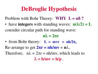
DeBroglie Hypothesis Problem with Bohr Theory: WHYL = n ? • have integers with standing waves: n(/2) = L consider circular path for standing wave: n = 2r • from Bohr theory: L = mvr = nh/2 Re-arrange to get 2r = nh/mv = n Therefore, n = 2r = nh/mv, which leads to = h/mv = h/p .
DeBroglie Hypothesis DeBroglie = h/mv = h/p In this case, we are considering the electron to be a WAVE, and the electron wave will “fit” around the orbit if the momentum (and energy) is just right(as in the above relation). But this will happen only for specific cases - and those are the specific allowed orbits (rn) and energies (En) that are allowed in the Bohr Theory!
DeBroglie Hypothesis The Introduction to Computer Homework on the Hydrogen Atom (Vol. 5, number 5) shows this electron wave fitting around the orbit for n=1 and n=2. What we now have is a wave/particle duality for light(E&M vs photon), AND a wave/particle duality for electrons!
DeBroglie Hypothesis If the electron behaves as a wave, with = h/mv, then we should be able to test this wave behavior via interference and diffraction. In fact, experiments show that electronsDO EXHIBIT INTERFERENCE when they go through multiple slits, just as the DeBroglie Hypothesis indicates.
DeBroglie Hypothesis Even neutrons have shown interference phenomena when they are diffracted from a crystal structure according to the DeBroglie Hypothesis: = h/p . Note that h is very small, so that normally will also be very small (unless the mv is also very small). A small means very little diffraction effects [1.22 = D sin()].
Quantum Theory What we are now dealing with is the Quantum Theory: • atoms are quantized (you can have 2 or 3, but not 2.5 atoms) • light is quantized (you can have 2 or 3 photons, but not 2.5) • in addition, we have quantum numbers (L = n , where n is an integer)
Heisenberg Uncertainty Principle There is a major problem with the wave/particle duality: • a wave with a definite frequency and wavelength (e.g., a nice sine wave) does not have a definite location. [At a definite location at a specific time the wave would have a definite phase, but the wave would not be said to be located there.] [ a nice travelling sine wave = A sin(kx-t)]
Heisenberg Uncertainty Principle b) A particle does have a definite location at a specific time, but it does not have a frequency or wavelength. c) Inbetween case: a group of sine waves can add together (via Fourier analysis) to give a semi-definite location: a result of Fourier analysis is this: the more the group shows up as a spike, the more waves it takes to make the group.
Heisenberg Uncertainty Principle A rough drawing of a sample inbetween case, where the wave is somewhat localized, and made up of several frequencies.
Heisenberg Uncertainty Principle A formal statement of this (fromFourier analysis) is: x * k (where k = 2/, and indicates the uncertainty in the value). But from the DeBroglie Hypothesis, = h/p, this uncertainty relation becomes: x * (2/) = x * (2p/h) = 1/2 , or x * p = /2.
Heisenberg Uncertainty Principle x * p = /2 The above is the BEST we can do, since there is always some experimental uncertainty. Thus the Heisenberg Uncertainty Principle says: x * p > /2 .
Heisenberg Uncertainty Principle A similar relation from Fourier analysisfor time and frequency:t * = 1/2leads to another part of the Uncertainty Principle (using E = hf):t * E > /2 . There is a third part: * L > /2 (where L is the angular momentum value). All of this is a direct result of the wave/particle dualityof light and matter.
Heisenberg Uncertainty Principle Let’s look at how this works in practice. Consider trying to locate an electron somewhere in space. You might try to “see” the electron by hitting it with a photon. The next slide will show an idealized diagram, that is, it will show a diagram assuming a definite position for the electron.
Heisenberg Uncertainty Principle We fire an incoming photon at the electron, have the photon hit and bounce, then trace the path of the outgoing photon back to see where the electron was. incoming photon electron
Heisenberg Uncertainty Principle screen slit so we can determine direction of the outgoing photon outgoing photon electron
Heisenberg Uncertainty Principle • Here the wave-particle duality creates a problem in determining where the electron was. photon hits here slit so we can determine direction of the outgoing photon electron
Heisenberg Uncertainty Principle • If we make the slit narrower to better determine the direction of the photon (and hence the location of the electron, the wave nature of light will cause the light to be diffracted. This diffraction pattern will cause some uncertainty in where the photon actually came from, and hence some uncertainty in where the electron was .
Heisenberg Uncertainty Principle We can reduce the diffraction angle if we reduce the wavelength (and hence increase the frequency and the energy of the photon). But if we do increase the energy of the photon, the photon will hit the electron harder and make it move more from its location, which will increase the uncertainty in the momentum of the electron.
Heisenberg Uncertainty Principle Thus, we can decrease the xof the electron only at the expense of increasing the uncertainty in pof the electron.
Heisenberg Uncertainty Principle Let’s consider a second example: trying to locate an electron’s y position by making it go through a narrow slit: only electrons that make it through the narrow slit will have the y value determined within the uncertainty of the slit width.
Heisenberg Uncertainty Principle But the more we narrow the slit (decrease y), the more the diffraction effects (wave aspect), and the more we are uncertain of the y motion (increase py) of the electron.
Heisenberg Uncertainty Principle Let’s take a look at how much uncertainty there is: x * p > /2 . Note that /2 is a very small number (5.3 x 10⁻³⁵ J-sec).
Heisenberg Uncertainty Principle If we were to apply this to a steel ball of mass .002 kg +/- .00002 kg, rolling at a speed of 2 m/s +/- .02 m/s, the uncertainty in momentum would be 4 x 10⁻⁷ kg*m/s . From the H.U.P, then, the best we could be sure of the position of the steel ball would be: x = 5.3 x 10⁻³⁵ J*s / 4 x 10⁻⁷ kg*m/s = 1.3 x 10⁻²⁸ m !
Heisenberg Uncertainty Principle As we have just demonstrated, the H.U.P. comes into play only when we are dealing with very small particles (like individual electrons or photons), not when we are dealing with normal size objects!
Heisenberg Uncertainty Principle If we apply this principle to the electron going around the atom, then we know the electron is somewhere near the atom, (x = 2r = 1 x 10⁻¹⁰ m) then there should be at least some uncertainty in the momentum of the atom: px > 5 x 10-35 J*s / 1 x 10⁻¹⁰ m = 5 x 10-25 m/s
Heisenberg Uncertainty Principle Solving for p = mv from the Bohr theory [KE + PE = Etotal, (1/2)mv2 - ke2/r = -13.6 eV gives v = 2.2 x 10⁶ m/s ] gives p = (9.1 x 10⁻³¹ kg) * (2.2 x 10⁶ m/s) = 2 x 10-24 kg*m/s; this means px is between -2 x 10-24 kg*m/s and 2 x 10-24 kg*m/s, with the minimum px being 5 x 10-25 kg*m/s, or 25% of p.
Heisenberg Uncertainty Principle Thus the H.U.P. says that we cannot really know exactly where and how fast the electron is going around the atom at any particular time. This is consistent with the idea that the electron is actually a wave as it moves around the electron.
Quantum Theory But if an electron acts as a wave when it is moving, WHAT IS WAVING? When light acts as a wave when it is moving, we have identified the ELECTROMAGNETIC FIELDas waving. But try to recall: what is the electric field? Can we directly measure it?
Quantum Theory Recall that by definition, E = F/q. We can only determine that a field exists by measuring an electric force! We have become so used to working with the electric and magnetic fields, that we tend to take their existence for granted. They certainly are a useful construct even if they don’t exist.
Quantum Theory We have four LAWS governing the electric and magnetic fields: MAXWELL’S EQUATIONS. By combining these laws we can get a WAVE EQUATIONfor E&M fields, and from this wave equation we can get the speed of the E&M wave and even more (such as reflection coefficients, etc.).
Quantum Theory But what do we do for electron waves? What laws or new law can we find that will work to give us the wealth of predictive power that MAXWELL’S EQUATIONS have given us?
Quantum Theory The way you get laws is try to explain something you already know about, and then see if you can generalize. A successful law will explain what you already know about, and predict things to look for that you may not know about. This is where the validity (or at least usefulness) of the law can be confirmed.
Quantum Theory Schrodinger started with the idea of Conservation of Energy: KE + PE = Etotal . He noted that • KE = (1/2)mv2 =p2/2m, and that =h/p, so that p = h/= (h/2)*(2/) = k = p, so KE = 2k2/2m • Etotal = hf= (h/2)*(2f)= .
Quantum Theory He then took a nice sine wave, and called whatever was waving, : (x,t) = A sin(kx-t) = Aei(kx-t) . He noted that both k and were in the exponent, and could be gotten down by differentiating. So he tried operators:
Quantum Theory (x,t) = A sin(kx-t) = Aei(kx-t). pop =i[d/dx]= i[-ikAe-i(kx-t)] = k = (h/2)*(2/)* = (h/ = p . similary: Eop= i[d/dt]= i[-iAei(kx-t)] = = ((h/2)*(2f)* = (hf = E .
Quantum Theory Conservation of Energy: KE + PE = Etotal becomes with the momentum and energy operators: -(2/2m)*(d2/dx2) + PE* = i(d/dt) which is called SCHRODINGER’S EQUATION. If it works for more than the free electron, then we can call it a LAW.
Quantum Theory What is waving here? What do we call ? the wavefunction Schrodinger’s Equation allows us to solve for the wavefunction. The operators then allow us to find out information about the electron, such as its energy and its momentum.
Quantum Theory To get a better handle on , let’s consider light: how did the E&M wave relate to the photon?
Quantum Theory The photon was the basic unit of energy for the light. The energy in the wave depended on the field strength squared. [Recall energy in capacitor, Energy = (1/2)CV2, where for parallel plates, Efield = V/d and C// = KoA/d, so that Energy = (1/2)*(KoA/d)*(Efieldd)2 = KoEfield2 * Vol, or Energy Efield2.]
Quantum Theory Since Energy is proportional to field strength squared, AND energy is proportional to the number of photons, THEN that implies that the number of photons is proportional to the square of the field strength. This then can be interpreted to mean that the square of the field strength is related to the probability of finding a photon.
Quantum Theory In the same way, the square of the wavefunction is related to the probability of find the electron! Since the wavefunction is a function of both x and t, then the probability of finding the electron is also a function of x and t! Prob(x,t) = (x,t)2
Quantum Theory Different situations for the electron, like being in the hydrogen atom, will show up in Schrodinger’s Equation in the PE part. Different PE functions (like PE = -ke2/r for the hydrogen atom) will cause the solution to Schrodinger’s equation to be different, just like different PE functions in the normal Conservation of Energy will cause different speeds to result for the particles.
Schrodinger’s Equation Let’s look at the case of an electron confined to a length, L, but otherwise free. We will first consider the 1-D case. Since the electron is free, PE=0. However, since it is confined to the length, L, we have boundary conditions: x=0,t) = 0, and(x=L,t) = 0.
Schrodinger’s Equation To solve this differential equation, we use the technique of separation of variables: (x,t) = X(x)*T(t). The partial derivative with respect to x does not affect T(t), and the partial derivative with respect to t does not affect X(x). We can also divide both sides of the equation by X(x)*T(t) to get:
Schrodinger’s Equation Note that theleft side depends solely on x, and the right side solely on t. This means that as far as x is concerned, the right side is a constant, and as far as t is concerned, the left side is a constant (which turns out to be the Energy).
Schrodinger’s Equation We now have two ordinary differential equations instead of one partial differential equation: -(2/2m)d2X/dx2 = E*Xfor X(x) i dT/dt = E*T for T(t). In fact, any situation where the PE does not explicitly depend on time will have this solution.
Schrodinger’s Equation i dT/dt = E*T for T(t) The above 1st order ordinary differential equation is easily solved if we recall that the differential of an exponential gives an exponential back again. So try T(t) = Aeat: i(aAeat) = E(Aeat) or ia = E, or a = E/i. But we know that E = , so this means that: a = /i = -i, and T(t) = A e-it.
Schrodinger’s Equation • Note that the probability depends on 2 (actually, since can be a complex quantity, Prob(x,t) = where is the complex conjugate of ). • Note also that T**T = Ae-it * Ae+it = A2 , but A can be incorporated as a constant into X(x). Thus the T part of can effectively be ignored if the PE does not depend on t.
Schrodinger’s Equation This means that when the PE does not depend on time, Schrodinger’s Equation can be re-written as (since iddt = E*) : (-2/2m)*d2/dx2 + PE* = E*. Note that can be complex (just like E could be written in complex form), but the Probability must be real (since it is a measurable quantity). Now we go on to the X equation.
Schrodinger’s Equation -(2/2m)d2X/dx2 = E*Xfor X(x) This equation can again be solved by inspection since we know that the second derivative of a sine (or cosine) function gives itself back again with a minus sign, so we’ll try X(x) = B sin(kx+φo): -(2/2m)(-Bk2 sin(kx+φo)) = E B sin(kx+φo) , or 2k2/2m = E (since p = k, E = p2/2m = KE but this is correct since PE = 0 in this case!)