Download
1 / 24
240 likes | 1.14k Views
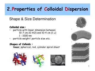
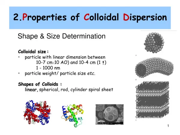
2. P roperties of C olloidal D ispersion. Shape & Size Determination. Colloidal size : particle with linear dimension between 10-7 cm ( 10 AO) and 10-4 cm (1 ) 1 - 1000 nm particle weight/ particle size etc. Shapes of Colloids : linear, spherical, rod, cylinder spiral sheet.

E N D
2.Properties of Colloidal Dispersion Shape & Size Determination Colloidal size: • particle with linear dimension between 10-7 cm (10 AO) and 10-4 cm (1 ) 1 - 1000 nm • particle weight/ particle size etc. Shapes of Colloids : linear, spherical, rod, cylinder spiral sheet
Molar Mass ( for polydispersed systems) • Number averaged • Weight averaged • Viscosity averaged • Surface averaged • Volume averaged • Second moment • Third moment • Radius of gyration n Number averaged Molar Mass
2.1 Colligative Propery In solution • Vapor pressure lowering P = ikpm • Boiling point elevation Tb = ikbm • Freezing point depression Tf = ikfm • Osmotic pressure = imRT (m = molality, i = van’t Hoff factor) In colloidal dispersion Osmotic pressure
Osmosis • the net movement of water across a partially permeable • membrane from a region of high solvent potential to an area of • low solvent potential, up a solute concentration gradient
Osmotic pressure • the hydrostaticpressure produced by a solution in a space • divided by a semipermeable membrane due to a differential in • the concentrations of solute For colloidal dispersion The osmotic pressure π can be calculated using the Macmillan & Mayer formula π = 1 [1 + Bc + B’c2 + …] cRT M M M2 = gh
Molar Mass Determination Dilute dispersion h = RT [1 + Bc ] c gM M Where c = g dm-3 or g/100 cm-3 M = Mn = number-averaged molar mass B = constants depend on medium h (cm g-1L) c Slope = intercept x B/Mn Intercept = RT g n c (g L-1)
Estimating the molar volume From the Macmillan & Mayer formula : B = ½NAVp where B = Virial coefficient NA = Avogadro # Vp = excluded volume, the volume into which the center of a molecule can not penetrate which is approximately equals to 8 times of the molar volume Example/exercise : Atkins
Osmotic pressure on bloodcells Donnan Equlibrium : activities product of ions inside = outside
Donnan equilibrium activity a = C Where a = activity = activity coefficient C = molar conc. log = - kz2 aNaCl, L = a NaCl, R (aNa+)L(aCl-)L = (a Na+ )R(a Cl-)R
Reverse Osmosis • a separation process that uses pressure to force a solvent • through a membrane that retains the solute on one side and allows • the pure solvent to pass to the other side Look for its application : drinking and waste water purifications, aquarium keeping, hydrogen production,car washing, food industry etc. Pressure
2.2 Kinetic property : Brownian Motion • either the random movement of particles suspended in a fluid or the mathematical model used to describe such random movements, often called a Wiener process. • The mathematical model of Brownian motion has several real-world applications. An often quoted example is stock market fluctuations. = 2Dt D = diffusion coefficient
2.2 Kinetic property :Diffusion the random walk of an ensemble of particles from regions of high concentration to regions of lower concentration
Einstein Relation (kinetic theory) where D= Diffusion constant, μ=mobility of the particles kB= Boltzmann's constant, and T=absolute temperature. The mobility μ is the ratio of the particle's terminal drift velocity to an applied force, μ= vd / F.
Diffusion of particles • For spherical particles of radius r, the mobility μ is the inverse of the frictional coefficient f, therefore Stokes law gives • f = 6r • where η is the viscosity of the medium. • Thus the Einstein relation becomes • This equation is also known as the Stokes-Einstein Relation.
Fick’s Law 1st Law • 1st law J = -D • 2nd law 2nd Law • where • Flux • mole m-2 s-1 • = molar concentration • = chemical potential D= diffusion coefficient
2.2 Kinetic property :Viscosity a measure of the resistance of a fluid to deform under shear stress • where: • is the frictional force, • r is the Stokes radius of the particle, • η is the fluid viscosity, and • is the particle's velocity.
Viscosity Measurement P R • = - PR4t 8VL = t o oto L • = viscosity of dispersion • o= viscosity of medium Unit:Poise (P)1 P = 1 dyne s-1 cm-2= 0.1N s m-2
Intermolecular forces • intermolecular forces are forces that act between stable molecules or between functional groups of macromolecules. • Intermolecular forces include momentary attractions between molecules, diatomic free elements, and individual atoms. • These forces includes London Dispersion forces, Dipole-dipole interactionsand Hydrogen bonding,.
Einstein Theory = o (1+2.5) • -1 = sp = 2.5 , sp : specific viscosity • o • = volume fraction of solvent replaced by solute molecule • = NAcVh MV where c = g cm-3 vh=hydrodynamic volume of solute
Einstein Theory = o (1+2.5) • -1 = sp = 2.5 , sp : specific viscosity • o • = NAcVh MV [] = lim sp= 2.5 , []: intrinsic viscosity c c [] = K(Mv)a Mark-Houwink equation K - types of dispersion a – shape & geometry of molecule
Assignment 2 (3-5 students per group) 1. At 25 oC D of Glucose = 6.81x10⁻¹⁰ m s-1 of water = 8.937x10³ P of Glucose = 1.55 g cm-3 Use the Stokes law to calculate the molecular mass of glucose, suppose that glucose molecule has a spherical shape with radius r 5 points
Assignment 2 2. Use the data below for Polystyrene in Toluene at 25 oC, calculate its molecular mass c/g cm-30 2.0 4.0 6.0 8.0 10.0 /10-4kg m-1s-15.58 6.15 6.74 7.35 7.98 8.64 Given :Kand a in the Mark-Houwink equation equal3.80x10-5 dm-3/g and 0.63, respectively (5 points) Due Date : 21 Aug 2009