LTL Decidability
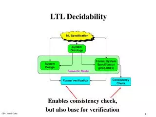
LTL Decidability. Enables consistency check, but also base for verification. A set is decidable if there is an effective procedure to decide whether an arbitrary element is a member of the set, or not. Effective Decision Procedure Termination .

LTL Decidability
E N D
Presentation Transcript
LTL Decidability Enables consistency check, but also base for verification Dr. Vered Gafni
A set is decidable if there is an effective procedure to decide • whether an arbitrary element is a member of the set, or not. • Effective Decision Procedure • Termination. • Soundness: if member returns yes. • Completeness: if returns yes then it is member. • In logic, decidability refers to the set of valid/satisfiable formulae • of a given logic. • f is satisfiable if I f for some interpratation I • f is valid if I f for all I ( f). • Recall, in logic Satisfiability Validity since • fis valid iff fis not satisfiable. Decidability Dr. Vered Gafni
Unsatisfiable Specification • During takeoff the system shall maintain the engine at 9000RPM. • Whenever the engine temperature exceeds 800°C the system • shall limit the engine to 5000RPM. The environment can produce input that makes it impossible to satisfy both requirements. Dr. Vered Gafni
Example: Propositional Calculus • Syntax (wff) · atoms: p, q, r,… and constant : tt, ff. · P, PQ, PQ, P Q, P Q • Semantics: an interpretation I: {p1,…,pk} {true, false}. · I tt, ff · I p iff I(p)=true · I P iff I P · I PQ iff I P or I Q Model equivalencies: PQ (P Q), PQP Q • Decidability:Check all possible interpretations (2n). Dr. Vered Gafni
Tableau Method: Satisfiability check for Prop. Calculus Satisfied iff A1 and A2are satisfied, both. Satisfied iff just B1 or B2 is satisfied Dr. Vered Gafni
Tableau Algorithm for a formula f • Construct a tree s.t. each node is labeled by a set Fsub(f)sub ( f) : 1. Start with the root node that contains f. 2. Repeat until nodes are closed or do not contain unchecked components that can be further decomposed (open node). - For every node that contains an unchecked -typeg constructa single subnode: F-{g} {g', A1(g), A2(g)} - For every node that contains an unchecked -typeg constructtwo sub-nodes: F-{g} {g', B1(g)}, F-{g} {g', B2(g)} - If any of the constructed nodes contains wffs g and g, markit closed, and do not continue expanding this node. • f is satisfiable iff there is an open leaf in the tree Dr. Vered Gafni
Examples (A B) C ((AB)C)’, (AB) ((AB)C)’, C ((AB)C)’, (AB)’, A, B A (B A) (A(BA))’, A, (BA) (A(BA))’, A, (BA)’,B (A(BA))’, A, ((BA))’, A Dr. Vered Gafni
Decision Procedure for LTL Satisfiability Recall, given LTL formula , • Satisfiability: . ? • Validity: . ? • Satisfiability Validity . . () . () • Outline of satisfiability algorithm • Construct directed-graph A, X • Search A, X tofind out whether it is -fulfilling • We prove that is satisfiable iff A, X is -fulfilling Dr. Vered Gafni
A,X Construction • Construct CL(): sub- formulae closure of . • Define Anodes as the consistent sub-sets of CL(). • Use ‘next’ relation to define the transitions Xover A. Dr. Vered Gafni
Closure of a Temporal Formula Examples of closures: CL() = { , ¬ | sub() } p • p • p • p • p • p • p • p • p • p • p • p • p • p • p • p • p • p • p • p • p • p • p • p CL()|2|| Assume any ¬¬ is replaced by (by ¬¬ equivalence rule) Dr. Vered Gafni
Example: CL((p q)) (p q) (p q) (p q) (p q) q p p q q q Dr. Vered Gafni
Atom hence, |D|=n, |A|2n where |CL()|=2n A set DCL() such that: • CL() D iff D • 12CL() 12D iff 1D or 2D • 1U2CL() • 1U2D 1Dor 2D • 2D 1U2D Completing for temporal derivatives yields: • CL() if D then D • = hence CL() if D then D • CL() if D then D • = hence CL() if D then D a maximal consistent set (w.r.t. satisfiability) of sub-formulae Dr. Vered Gafni
Atom Examples (I) Cl(p)={p,p}: p p Cl(Op)={Op, p, O(p), p}: O(p), p Op,p O(p), p O(p), p CL(p)={ p, p, p, p }: p, p p, p p, p CL(p)= {p,p, p, p}: p, p p, p p, p Dr. Vered Gafni
Atoms Examples (II) CL(p)={p, p, p, p, p, p } p,p, p p,p, p p,p, p p, p, p p, p, p Cl(pq}={pq, p, q , q, (pq), p, q, q} pq, p,q, q pq, p,q, q pq, p,q, q pq, p,q, q pq, p,q, q pq, p,q, q Dr. Vered Gafni
LTL Graph of -graph is a directed A, X where • A is the set of Atoms of • X is a “next” relation defined as follows: • OCL(), OD1 iff D2 • 1U2CL(), • if 1U2,2D1 then 1U2 D2 • if 1U2D2, 1D1 then 1U2D1 (D1,D2)X 1U2,2 1U2 O 1U2, 1 1U2 Dr. Vered Gafni
LTL Graph of • 1U2CL(), • if 1U2,2D1 then 1U2 D2 • if 1U2D2, 1D1 then 1U2D1 (D1,D2)X Derived constraints • CL(): if ,D1 then D2 • if D2 then D1 • CL(): if ,D1 then D2 • if D2 then D1 • CL(): if D1 then D2 • CL(): if D1 then D2 Dr. Vered Gafni
Graph Examples (I) Cl(p)={p,p} p p Cl(Op)={Op, p, O(p), p} O(p), p Op,p, O(p), p O(p), p Dr. Vered Gafni
Graph Examples (II) CL(p)={ p, p, p, p } CL(), ,D1D2 D2D1 p, p p, p p1 p1 p, p CL(), D1D2 , D1 D2 p2 CL(p)= {p,p, p, p} p, p p2 p2 p2 p, p p, p Dr. Vered Gafni
Graph Example p CL(p)={ p, p, p, p, p, p } p,p, p p,p, p • CL(), • ,D1D2 • D2D1 • CL(), • D1D2 • CL(): • if D1D2 p,p, p p, p, p p, p, p Dr. Vered Gafni
Graph Example: p CL(p)={ p, p, p, p, p, p } p,p, p p,p, p • CL(), • ,D1D2 • D2D1 • CL(), • ,D1D2 • D2D1 p,p,p p,p,p p, p, p Dr. Vered Gafni
Fulfilling Path An infinite path D0, D1, … in A, X is -fulfilling path iff • D0 • i0, if UDi then ji s. t. Dj Claim 1: U ( O(U)) -- exercise Claim 2: Let D0, D1, … be a -fulfilling path in A, X then UDi iff ki s. t. Dk and Dj, j=i..k-1 Dr. Vered Gafni
Satisfiability in A, X Theorem 1: A formula is satisfiable iff there is a -fulfilling path in A, X Proof (principle): Let be a model of , define a sequence D0,D1,… s.t. Di={ CL() | i |= }. Show that: • Di are atoms, and (Di,Di+1 )X • the sequence forms a -fulfilling path in A, X Conversely, given D0,D1,…, a -fulfilling path in A, X , define a trace 0, 1,… s.t. pi iff pDi. Show that |= (induction on the structure of ). Dr. Vered Gafni
Part A: satisfiable there is a -fulfilling path in A, X Proof: Let be a model of . Define a sequence D0,D1,… s.t. Di={CL() | i|= }. We show that: Di are atoms: • i|= iff i|¬ (sem.), • i|= iffi|=or i|=(sem.). 3.1) UDi def i|=U+(2) i|=O(U) or i|= sem i|= or i|= def Dior Di 3.2) Di def i|= sem i|=Udef UDi U (O(U)) • Atom definition: • if UD then Dor D, • If D then UD Dr. Vered Gafni
OD1 iff D2 U,D1UD2; UD2, D1UD1. U (O(U)) (Di,Di+1 )X: ODi def i|=O() sem i+1|=def Di+1. U,Di def i|=U +log i|=O(U) or i|= sem i|=O(U) sem i|=O(U) sem i+1|=Udef UDi+1. U Di+1, Di def i+1|=U and i|=sem i|=O(U) and i|= sem i|=O(U) sem i|= (O(U)) sem i|=Udef UDi. Fulfillness: - UDi def i|=Usem ji s.t. j|= defDj . - by definition if be a model of then 0|= hence D0 Proof part A : (cont.) Dr. Vered Gafni
Part B: There is a -fulfilling path in A, X is satisfiable Proof : Let D0,D1,… be -fulfilling path in A,X . Define a trace where i={ pDi | p proposition }. Show by Ind. on the structure of that CL(), Dii|=. - pDidef.pisem. i|=p. - DiatomDiind.i| sem. i|=. - DiatomDi or Diind.i|=, or i|= sem.i|= - ODiX Di+1ind.i+1|= sem.i|=O - UDi ki s. t. Dk and Dj, j=i..k-1 {fulfilling+claim 2} ki s. t. k|= & ijk, j|= {induction} i|=U {semantics} Finally, |= since D0 therefore is satisfiable. Dr. Vered Gafni
Decision Algorithm Following Theorem 1, we propose the following algorithm: • Given LTL formula, ,construct the graph A,X , where: - A is the set of atoms of , - X is the next relation • Find whether or not, A, X spans a -fulfilling path. Dr. Vered Gafni
Strongly Connected Graph A graph is strongly connected (s.c.) if from every node there is a path to every other node. From Graph Theory: Every graph is decomposable into maximal s.c. components (s.c.c) s.t. the connection between the components is acyclic. Dr. Vered Gafni
p, p p, q p q Identifying -fulfilling path in G[] = A,X A sub-graph CG[] is self-fulfilling if it is s.c. and for every formula U that belongs to an atom DC there is an atom EC such that E. Theorem 2: G[] spans a -fulfilling path iff G[] contains a sub-graph that is: • self-fulfilling • reachable from an atom that contains . Dr. Vered Gafni
inf() vs. -fulfilling path Let =A0,A1,… be an -path in G[] s.t. A0. Define inf() = { the set of Atoms that appear i.m. times in } Claim: If inf()is self-fulfilling then is -fulfilling path. Dr. Vered Gafni
Proof: inf() vs. -fulfilling path Let =A0,A1,… be an -path in G[] s.t. A0. Define inf() = { the set of Atoms that appear i.m. times in } Claim: If inf()is self-fulfilling then is -fulfilling path. Proof: Let Am s.t.UAm. Then, • Aminf()s.f. Binf() s.t. B inf jm. B=Aj • Aminf(). k>m s.t. nk Aninf(). • If mik s.t. Aiwe are finished. • o.w. mik, U,Ai (X relation). So, UAk and then by (1). Dr. Vered Gafni
Theorem 2: Part 1: If CG[] is self-fulfilling and reachable from atom I s.t. I then G[] spans a -fulfilling path. Dr. Vered Gafni
Theorem 2: Proof Part 1: If CG[] is self-fulfilling and reachable from atom I s.t. I then G[] spans a -fulfilling path. Proof: CG[] is reachable from Ihence there exists in G[] a finite path D0,…,Dks.t. k≥0, D0=I (hence D0), and Dk C (1st). Let U= D0,…,Dk-1 if k≥1, o.w. the empty sequence. C is s.c. (def, of s.f.) hence there exists in Ca path W=A1,A2,…,Ans.t.A1=An=Dk, (Ai,Ai+1)X , and W traverses all the Atoms in C. Let =(U,W), then (by construction): inf()={A | A appears in W} = {A | AC} Hence, inf() is self-fulfilling (as C is given to be self-fulfilling). Therefore, by previous claim is a -fulfilling path. Dr. Vered Gafni
Theorem 2: Proof Part B: if G[] spans a -fulfilling path=D0,D1,… then G[] contains a sub-graph C that is self-fulfilling and reachable from D0 (an Atom that contains ). Proof: Define C=inf(). 1. Let m be the minimal index s.t. for every nm Dninf(). Hence, inf()is reachable from D0 (an Atom that contains ) by D0…Dm. 2,inf() is self-fulfilling (proof follows). Dr. Vered Gafni
Claim: If a path is -fulfilling then inf() is self-fulfilling. Proof: • inf() is s.c.: • A,Binf() ∞ji. Dji=A, and ∞ki. Dki=B. • Let m be minimal s.t. nm Dninf(). Thus, jlm kh s.t. mjlkh. Namely: DjlDkh is a path ininf() s.t. Djl=A, Dkh=B. • Let Ainf() s.t. UA, consider the first index of A in s.t. in the sequel all elements are in inf()(1) then since is -fulfilling path it has a future atom B s.t. B. But Binf() by (1) Dr. Vered Gafni
LTL Decidability Theorem: LTL satisfiability (hence validity) is decidable. Proof: • is satisfiable iff there is a -fulfilling path in G[] (Theorem 1) • G[] spans a -fulfilling path iff G[] contains a sub graph that is self-fulfilling and reachable from an atom that contains . (Theorem 2). • Self-fulfillness in G[] isdecidable • Decomposition into s.c.c. (Graph Theory) • Temporal commitment of U (finite check) • Reachability in G[] is decidable (trivial). Dr. Vered Gafni
Decision Procedure Algorithm • Decompose A,X into maximal* s.c. components. Call a maximal s.c.c. CA,X uselessif: • C is not reachable from an Atom that contains (could be C itself), or • C is not self fulfilling • Check every terminal component. If it is useless remove it. • If all components have been removed then there is no model. • Otherwise, a terminal s.c.c C that is not useless has been reached, then every path that starts in an atom that contains , and enters Cand travels infinitly often through every state C, defines a model. * Claim: Let CC’ s.c. components.If C is self-fulfilling so is C’. A,X may consist of a number of disconnected subgraphs Dr. Vered Gafni
Satisfiability Graphs Examples (I) p p, p p, p p, p p, p useless p p, p p, p Dr. Vered Gafni
Graph Example p useless –not self-fulfilling p,p, p p,p, p p,p, p useless – no access from initial node p, p, p p, p, p Dr. Vered Gafni
Graph Example: p p,p, p p,p, p p,p,p useless p,p,p p, p, p Dr. Vered Gafni
Graph Example: (p q) (p q) (p q) p, q, q (p q) (p q) p, q, q (p q) (p q) p, q, q (p q) (p q) p, q, q (p q) (p q) q, p, q (p q) (p q) q, p, q (p q) (p q) p, q, q (p q) (p q) p, q, q Dr. Vered Gafni
Graph Example: pUq q useless pUq q, (pUq q) pUq, (pUq), q, q, p, p, q , q pUq q, q, pUq, p, q (pUq q) (pUq) q, p, q (pUq q) (pUq) q, p, q (pUq q) (pUq) q, p, q (pUq q) (pUq) q, p, q (pUq q) (pUq) q, p, q useless Dr. Vered Gafni
Algorithm Complexity • Time bound: 2O(||). • |A|≤2||, hence |G[]|≤22||. • Decomposition of G[] into s.c.c. : O|G[]|. • All required checking: time linear in |A|||. • PSPACE-complete Dr. Vered Gafni
On the Fly Graph Construction contains Reminder: LTL Formula Each node is a set of consistent sub-formulae of Search for fulfilling path Dr. Vered Gafni
On the Fly Graph Construction Idea: save node development by: • Avoid development of sub-graphs that are not reachable from a root Atom. • Let nodes represent equivalence classes of Atoms. Dr. Vered Gafni
On the Fly Graph Construction p Examples of possible sub-graphs elimination. p,p, p p,p, p p,p, p p, p, p p, p, p p p, p p, p p, p Dr. Vered Gafni
On the Fly Graph Construction Examples of Atoms’ equivalence classes. O(p), p Op,p, Op O(p), p O(p), p All atoms that contain the specified formulae Op p tt,O(tt) Dr. Vered Gafni
On the Fly Construction Idea • Start with constructing Atoms that contain the original formula. • For each Atom construct only Atoms that fulfill the next conditions for this Atom, and connect them. • While construction identify Atoms that completely agree on their successors. Dr. Vered Gafni
On the Fly Graph Construction Algorithm Step 1: Raw graph construction 1. Start with a root node that consists of: . 2. Use , rules as long as possible. 3. Close nodes that contain formulae of the form: p,p. 4. Close all nodes which all of their off-springs are closed. 5. For every open leaf that contains “next” conditions: (and may be other formulae) define a sub-node that consists of the promised formulae. If such node already exists in the graph connect the worked out node to that node, otherwise construct a new node. 6. Return to 2. Dr. Vered Gafni
Extended -typeclassification Dr. Vered Gafni
Extended typeclassification Dr. Vered Gafni