Download

1 / 17
170 likes | 553 Views
AAEC 4302 ADVANCED STATISTICAL METHODS IN AGRICULTURAL RESEARCH. Part II: Theory and Estimation of Regression Models Chapter 5: Simple Regression Theory. Population Line:. E[Y] = B 0 +B 1 X. Y i = E[Y i ]+u i. u i. E[Y i ] = B 0 +B 1 X i. Xi. Population Line:. E[Y] = B 0 +B 1 X. ^.

E N D
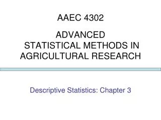
AAEC 4302ADVANCED STATISTICAL METHODS IN AGRICULTURAL RESEARCH Part II: Theory and Estimation of Regression Models Chapter 5: Simple Regression Theory
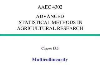
Population Line: E[Y] = B0+B1X Yi = E[Yi]+ui ui E[Yi] = B0+B1Xi Xi
Population Line: E[Y] = B0+B1X ^ Yi = Yi + ei Estimated Line: ^ ^ ^ Y = B0+B1X ei ui ^ ^ ^ Yi = B0+B1Xi E[Yi] Xi
^ ^ ^ Y = B0+B1X ei ei ei ei ei ei Xi
The Ordinary Least Squares (OLS) Method • In the Ordinary Least Squares (OLS) method, the criterion for estimating β0 and β1 is to make the sum of the squared residuals (SSR) of the fitted regression line as small as possible i.e.:Minimize SSR = minimize = minimize = minimize
The Ordinary Least Squares (OLS) Method • The OLS estimator (formulas) are: (5.12) (5.13)
The Ordinary Least Squares (OLS) Method • The regression line estimated using the OLS method has the following key properties: • (i.e. the sum of its residuals is zero) • It always passes through the point • The residual values (ei’s) are not correlated with the values of the independent variable (Xi’s)
Interpretation of the Regression Model • Assume, for example, that the estimated or fitted regression equation is: • or • Yi = 3.7 + 0.15Xi + ei
Interpretation of the Regression Model Yi = 3.7 + 0.15Xi + ei • The value of = 0.15 indicates that if the average cotton price received by farmers in the previous year increases by 1 cent/pound (i.e. X=1), then this year’s cotton acreage is predicted to increase by 0.15 million acres (150,000 acres).
Interpretation of the Regression Model Yi = 3.7 + 0.15Xi + ei • The value of = 3.7 indicates that if the average cotton price received by farmers in the previous year was zero (i.e. =0), the cotton acreage planted this year will be 3.7 million (3,700,000) acres; sometimes the intercept makes no practical sense.
Measures of Goodness of Fit • There are two statistics (formulas) that quantify how well the estimated regression line fits the data: • The standard error of the regression (SER)(Sometimes called the standard error of the estimate) • R2 - coefficient of determination
Measures of Goodness of Fit • The SER slightly differs from the standard deviation of the ei’s (by the degrees of freedom): (5.20)
Measures of Goodness of Fit: The R2 • The term on the left measures the proportion of the total variation in Y not explained by the model (i.e. by X) • Thus, the R2 measures the proportion of the total variation in Y that is explained by the model (i.e. X)
Properties of the OLS Estimators • The Gauss-Markov Theorem states the properties of the OLS estimators; i.e. of the: and They are unbiased E[B0 ]= and E[B1]=
Properties of the OLS Estimators If the dependent variable Y (and thus the error term of the population regression model, ui) has a normal distribution, the OLS estimators have the minimum variance
Properties of the OLS Estimators • BLUE – Best Linear Unbiased Estimator • Unbiased => bias of βj = E(βj ) -βj = 0 • Best Unbiased => minimum variance & unbiased • Linear => the estimator is linear ^ ^