Optimization Methods
560 likes | 833 Views
Optimization Methods. REM 658: Energy and Materials Systems Modeling January 24, 2008. Optimization Methods. Used to find a maximizing or minimizing outcome for a problem, subject to constraints (i.e. scarce resources) Maximize profit, utility Minimize cost, labor

Optimization Methods
E N D
Presentation Transcript
Optimization Methods REM 658: Energy and Materials Systems Modeling January 24, 2008
Optimization Methods • Used to find a maximizing or minimizing outcome for a problem, subject to constraints (i.e. scarce resources) • Maximize profit, utility • Minimize cost, labor • A variety of applications including: • Allocating production effort • Choosing a mix of investments • Transportation logistics • Professional sports schedules • Energy-specific applications (e.g. refinery product mix, electricity dispatch) • Also may be called mathematical programming, operations research, industrial engineering, ...
Optimization Methods • All optimization problems have one objective function, as well as decision variables and constraints • If the objective function and constraints are linear, the problem can be solved using linear methods (a.k.a. linear programming) • Some problems require non-linear methods • Loss of radio signal strength with distance in microwave communications • Economies of scale and learning • Non-linear programming is more complex and it is more difficult to achieve a single optimal solution
Linear ProgrammingOutline • Formulating a LP problem • Checking LP assumptions • Solving the LP problem • Potential Solution Problems • Analyzing the Solution
LP Problem Formulation Problem Formulation - translating information about the problem into a system of linear equations. • Identify the problem objective. • Identify the decision variables. • Identify the constraints. • Write the objective function and constraints in terms of the decision variables. • Add any implicit constraints, such as non-negative restrictions. • Arrange the system of equations in a consistent form suitable for solving.
Linear ProgrammingExample 1 – Apple Profits “I am a manager at an Apple manufacturer in Asia. We specialize in making iPods and iPhones. The business objective is to maximize profits. Steve Jobs just asked us how much of each product will we be producing this week, and what kind of profits he can expect to pocket.’’
Recall: LP Problem Formulation Problem Formulation - translating information about the problem into a system of linear equations. • Identify the problem objective. • Identify the decision variables. • Identify the constraints. • Write the objective function and constraints in terms of the decision variables. • Add any implicit constraints, such as non-negative restrictions. • Arrange the system of equations in a consistent form suitable for solving.
Example 1 – Apple Profits • Identify the problem objective: • To maximize profits from manufacturing iPods and iPhones. • Each iPod is associated with a net profit of $75; Each iPhone with a net profit of $100. • Identify decision variables: • Number of iPods and iPhones to produce.
Recall: LP Problem Formulation Problem Formulation - translating information about the problem into a system of linear equations. • Identify the problem objective. • Identify the decision variables. • Identify the constraints. • Write the objective function and constraints in terms of the decision variables. • Add any implicit constraints, such as non-negative restrictions. • Arrange the system of equations in a consistent form suitable for solving.
Example 1 – Apple Profits • Identify the constraints: • Total assembly time is limited to 9,000 hours per week. Each iPhone takes 3 hours to assemble and an iPod 2 hours. • Raw material supply is limited to 5,000 PCBs per week. Each iPhone needs 2 PCBs, whereas an iPod needs only 1. • Consumers demand a minimum of 500 iPhones and 3000 iPods per week.
Recall: LP Problem Formulation Problem Formulation - translating information about the problem into a system of linear equations. • Identify the problem objective. • Identify the decision variables. • Identify the constraints. • Write the objective function and constraints in terms of the decision variables. • Add any implicit constraints, such as non-negative restrictions. • Arrange the system of equations in a consistent form suitable for solving.
Example 1 – Apple Profits • Write the objective function and constraints in terms of the decision variables: Recall: I want to maximize Steve Jobs’ profit! How many iPhones and iPods should I make this week? Net profit gained from selling a iPhone is $100 Net profit gained from selling a iPod is $75 • Decision Variables • Let x1 = iPhones • x2= iPods • Objective Function • Let z = profit • Thus, • Max. z = 100x1 + 75x2 Objective Function Coefficients
Example 1 – Apple Profits • Write the objective function and constraints in terms of the decision variables, cont’d: Technological Coefficients • Recall: • Total assembly time is limited to 9,000 hours per week. Each iPhone takes 3 hours to assemble and an iPod 2 hours. • PCB supply is limited to 5,000 PCBs per week. Each iPhone needs 2 PCBs, whereas an iPod needs only 1. • Consumers demand a minimum of 500 iPhones and 3,000 iPods. 3x1 + 2x2 <= 9,000 2x1 + x2 <= 5,000 x1 >= 500 x2 >= 3,000 • Step 5: Implicit constraints (non-negative decision variables) x1, x2 >= 0
Recall: LP Problem Formulation Problem Formulation - translating information about the problem into a system of linear equations. • Identify the problem objective. • Identify the decision variables. • Identify the constraints. • Write the objective function and constraints in terms of the decision variables. • Add any implicit constraints, such as non-negative restrictions. • Arrange the system of equations in a consistent form suitable for solving.
Example 1 – Apple Profits • Arrange the system of equations in a consistent form suitable for solving. • Three ways of solving a linear programming model: • Graphically • Algebraically (Simplex Algorithm) • Computer program (Excel Solver)
6000 Min i Phones 5000 Feasible Region • Graphical Solution 4000 Min i Pods i Pods 3000 2000 PCB Constraint 1000 Assembly Constraint 0 0 1000 2000 3000 4000 i Phones
Example 1 – Apple Profits • Arrange the system of equations in a consistent form suitable for solving. • Algebraic Solution Maximize: z = 100x1 + 75x2 Subject to: 3x1 + 2x2 <= 9,000 2x1 + x2 <= 5,000 x1 >= 500 x2 >= 3,000 x1, x2 >= 0 Algebraic formulations use the Simplex algorithm
Example 1 – Apple Profits • Arrange the system of equations in a consistent form suitable for solving. • Computational Solution (Solver)
Example 1 – Apple Profits Checking LP Assumptions • Linearity • Proportionality • Additivity • Divisibility • Certainty Maximize: z = 100x1 + 75x2 Subject to: 3x1 + 2x2 <= 9,000 2x1 + x2 <= 5,000 x1 >= 500 x2 >= 3,000 x1, x2 >= 0
Optimal Solution Feasible Solution Solving the LP Problem Min i Phones Feasible Region • Graphical Solution Min i Pods PCB Constraint Assembly Constraint Isoprofit Line
Example 1 – Apple Profits: Solving the LP Problem • Algebraic Solution (Simplex Algorithm) Solution Profit: z = $331,250 Variables: x1 = 500, x2 = 3,750 Constraints: 3x1 + 2x2 = 9,000 (<= 9,000) 2x1 + x2 = 4,750 (<= 5,000) x1 = 500 (>= 500) x2 = 3,750 (>= 3,000) x1, x2 >= 0 http://optlab-server.sce.carleton.ca/POAnimations2007/CornerPoint.html
Example 1 – Apple Profits: Solving the LP Problem • Computational Solution 3,750 iPods Total Profit 500 iPhones
Linear ProgrammingSolution Problems Unbounded Feasible Region No Feasible Solution Infinite Solutions
Linear Programming(Special Cases - Example 1) I drink juice and water. 1 glass of juice is equivalent to ½ glass of water in terms of hydration. I want to maximize my daily hydration so that I can study. We need to drink at least 8 glasses of liquid a day. Let: z = hydration x1 = water x2 = juice Max. z = x1 + 0.5(x2) Subject to: x1 + x2 >= 8 x1,x2 >= 0 How many glasses of water and juice should I drink each day?
Linear Programming(Special Cases - Example 2 - Paulus’ Wedding Conundrum) We want to minimize the cost of our reception We need to invite the immediate family, plus the extended family and friends The immediate family goes to 2 receptions (lunch and dinner) The extended family and friends goes to dinner only The cost of meals is on average, $50/person Constraints: We are willing to spend $2000 on immediate family, and $2000 on extended + friends Parents’ expectation: Immediate family has at least 60 people Want to invite at least 40 of their friends Dinner reception: The restaurant won’t book us unless there are at least 50 people. Let x1 = immediate family Let x2 = extended family and friends Let Z = cost of reception Min. Z = $50 (2x1 + x2) s.t. $50 ( 2x1 ) <= $2000 $50 (x2) <= $2000 x1 >= 60 x2 >= 40 x1 + x2 >= 50 x1, x2 >= 0 Who should I invite?
Analyzing the SolutionBinding Constraints and Slack Variables • Binding Constraint • A constraint is binding when relaxing it changes the optimal solution. • Slack variable • The value of the slack variable indicates the change in the constraint that would lead it to become binding. Value is zero for binding constraints.
Optimal Solution Feasible Solution Solving the LP Problem Min i Phones Feasible Region • Graphical Solution Min i Pods PCB Constraint Assembly Constraint Isoprofit Line
Example 1 – Apple Profits: Analyzing the SolutionBinding Constraints and Slack Variables Solution Profit: z = $331,250 Variables: x1 = 500, x2 = 3,750 Subject to: 3x1 + 2x2 = 9,000 (<= 9,000) 2x1 + x2 = 4,750 (<= 5,000) x1 = 500 (>= 500) x2 = 3,750 (>= 3,000) x1, x2 >= 0 Binding, Assembly Non Binding, PCBs Binding, Demand for iPhones Non Binding, Demand for iPods Non Binding, (Intuitive)
Analyzing the SolutionShadow Price • The amount by which the solution value of the objective function increases (or decreases) for a one-unit relaxation in the right-hand-side of a given constraint. • Each constraint has a shadow price. • Indicates the marginal cost of a constraint (also called the dual value). • Value is zero for non-binding constraints.
Example 1 – Apple Profits: Analyzing the SolutionShadow Price Solution Profit: z = $331,250 Variables: x1 = 500, x2 = 3,750 Subject to: 3x1 + 2x2 = 9,000 (<= 9,000) 2x1 + x2 = 4,750 (<= 5,000) x1 = 500 (>= 500) x2 = 3,750 (>= 3,000) x1, x2 >= 0 Shadow Price = $37.5 / hour Shadow Price = $0 / PCB Shadow Price = -$12.5 / iPhone Shadow Price = $0 / iPod
Analyzing the SolutionReduced Cost • Reduced Cost • The amount by which the objective function will change if a decision variable is forced to non-zero. • The amount by which the variable's objective function coefficient (often cost) would need to change in order for the variable to enter the solution. • Value is zero for variables that already enter the solution.
Sensitivity Analysis • Study of how the optimal solution to an optimization problem changes given changes in the coefficients (objective function and technological). • Helps decision makers decide which uncertain coefficients have the greatest impact on the outcome. • May direct future research to address uncertainties. • May affect the decision depending on the assessment of risk.
Threshold Analysis • Establishing critical values (desired or undesired) for the optimal solution and doing sensitivity analysis to determine the conditions under which the thresholds they represent are crossed. • Atmospheric CO2: 550 ppm • GHG abatement cost: $100/tonne
What is MARKAL? • Optimization model of the energy system • Uses linear programming • Technologically explicit • A very large set of technologies • Technical data (financial cost) required to describe each technology • Existing technologies and those expected to be available • Dynamic • Tracks technologies over time (up to nine five-yr periods)
What is MARKAL? Cont’d • Partial equilibrium (“integrated”) • Feedbacks between energy supply and demand • Feedbacks between the integrated energy system and the economy as a whole • SAGE variant introducing more behavioral realism • Myopic economic agents • Market sharing algorithm • Consists of software plus specific database • Used in North America, Europe, elsewhere • Typical model has 4,000 to 6,000 variables plus a comparable number of equations!
Decision Variables • Decision variables • Variables representing energy carriers • Quantity of each energy form available in each period • Variables related to energy supply technologies • New investment in each technology in each time period • Installed capacity of each technology in each time period • Utilized capacity of each technology in each time period • Variables related to demand technologies • Model finds the best set of energy technologies (extraction, transport, conversion, and use) and energy flows
Objective Function, Constraints • Objective function • Minimize total discounted net present cost of the energy system over the planning horizon, OR • Minimize weighted function of cost and environmental emissions (can include supply security as well) • Constraints • Satisfaction of useful demand (NOT final energy consumption) • Fuel balances • Limit on operations • Period-to-period capacity conservation • Bounds on market penetration of individual technology • Others, such as maximum allowable emissions
Emission Reductions • Emission reductions may be treated as either • A constraint (corresponds to establishing regulations on emissions), OR • As part of the objective function (corresponds to a “carbon tax”)
Strengths/Appropriate Uses • Powerful tool for decision-making • Decision-maker has CONTROL over decision variables • Prescriptive/normative analysis • Applications we have talked about before… • Capable of dealing with very complex systems • Can find an optimal equilibrium throughout an entire system
Weaknesses/Inappropriate Uses • Only useful for forecasting (descriptive/positive analysis) if real economic agents (decision makers) are “optimizers” • Conventional bottom-up optimization models of the energy system lack behavioral realism • Assume perfect information across time and space • Decisions based on financial costs only • Assume agents are homogeneous • Penny switching solutions • Low cost estimates for GHG emission reduction • Conventional models lack equilibrium feedbacks
For More Information • The Journal of Operations Research • Practical Optimization: A Gentle Introduction by John W. Chinneckhttp://www.sce.carleton.ca/faculty/chinneck/po.html