Download
1 / 89
890 likes | 908 Views
Learn how decision tree classification is used in machine learning, using bat call data as an example. Explore the process of constructing a decision tree and the concept of information gain.

E N D
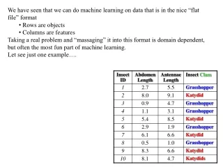
We have seen that we can do machine learning on data that is in the nice “flat file” format • Rows are objects • Columns are features • Taking a real problem and “massaging” it into this format is domain dependent, but often the most fun part of machine learning. • Let see just one example….
(Western Pipistrelle (Parastrellushesperus) Photo by Michael Durham
A spectrogram of a bat call. Western pipistrelle calls
We can easily measure two features of bat calls. Their characteristic frequency and their callduration Characteristic frequency Call duration
Classification • We have seen 2 classification techniques: • Simple linear classifier, Nearest neighbor,. • Let us see two more techniques: • Decision tree, Naïve Bayes • There are other techniques: • Neural Networks, Support Vector Machines, … that we will not consider..
I have a box of apples.. 1 H(X) Pr(X = good) = p then Pr(X = bad) = 1 − p the entropy of X is given by 0.5 0 0 binary entropy function attains its maximum value when p = 0.5 1 All good All bad
Decision Tree Classifier 10 9 8 7 6 5 4 3 2 1 1 2 3 4 5 6 7 8 9 10 Ross Quinlan Abdomen Length > 7.1? Antenna Length yes no Antenna Length > 6.0? Katydid yes no Katydid Grasshopper Abdomen Length
Antennae shorter than body? Yes No 3 Tarsi? Grasshopper Yes No Foretiba has ears? Yes No Cricket Decision trees predate computers Katydids Camel Cricket
Decision Tree Classification • Decision tree • A flow-chart-like tree structure • Internal node denotes a test on an attribute • Branch represents an outcome of the test • Leaf nodes represent class labels or class distribution • Decision tree generation consists of two phases • Tree construction • At start, all the training examples are at the root • Partition examples recursively based on selected attributes • Tree pruning • Identify and remove branches that reflect noise or outliers • Use of decision tree: Classifying an unknown sample • Test the attribute values of the sample against the decision tree
How do we construct the decision tree? • Basic algorithm (a greedy algorithm) • Tree is constructed in a top-down recursive divide-and-conquer manner • At start, all the training examples are at the root • Attributes are categorical (if continuous-valued, they can be discretized in advance) • Examples are partitioned recursively based on selected attributes. • Test attributes are selected on the basis of a heuristic or statistical measure (e.g., information gain) • Conditions for stopping partitioning • All samples for a given node belong to the same class • There are no remaining attributes for further partitioning – majority voting is employed for classifying the leaf • There are no samples left
Information Gain as A Splitting Criteria • Select the attribute with the highest information gain (information gain is the expected reduction in entropy). • Assume there are two classes, P and N • Let the set of examples S contain p elements of class P and n elements of class N • The amount of information, needed to decide if an arbitrary example in S belongs to P or N is defined as 0 log(0) is defined as0
Information Gain in Decision Tree Induction • Assume that using attribute A, a current set will be partitioned into some number of child sets • The encoding information that would be gained by branching on A Note: entropy is at its minimum if the collection of objects is completely uniform
Entropy(4F,5M) = -(4/9)log2(4/9) - (5/9)log2(5/9) = 0.9911 no yes Hair Length <= 5? Let us try splitting on Hair length Entropy(3F,2M) = -(3/5)log2(3/5) - (2/5)log2(2/5) = 0.9710 Entropy(1F,3M) = -(1/4)log2(1/4) - (3/4)log2(3/4) = 0.8113 Gain(Hair Length <= 5) = 0.9911 – (4/9 * 0.8113 + 5/9 * 0.9710 ) = 0.0911
Entropy(4F,5M) = -(4/9)log2(4/9) - (5/9)log2(5/9) = 0.9911 no yes Weight <= 160? Let us try splitting on Weight Entropy(0F,4M) = -(0/4)log2(0/4) - (4/4)log2(4/4) = 0 Entropy(4F,1M) = -(4/5)log2(4/5) - (1/5)log2(1/5) = 0.7219 Gain(Weight <= 160) = 0.9911 – (5/9 * 0.7219 + 4/9 * 0 ) = 0.5900
Entropy(4F,5M) = -(4/9)log2(4/9) - (5/9)log2(5/9) = 0.9911 no yes age <= 40? Let us try splitting on Age Entropy(1F,2M) = -(1/3)log2(1/3) - (2/3)log2(2/3) = 0.9183 Entropy(3F,3M) = -(3/6)log2(3/6) - (3/6)log2(3/6) = 1 Gain(Age <= 40) = 0.9911 – (6/9 * 1 + 3/9 * 0.9183 ) = 0.0183
Of the 3 features we had, Weight was best. But while people who weigh over 160 are perfectly classified (as males), the under 160 people are not perfectly classified… So we simply recurse! no yes Weight <= 160? This time we find that we can split on Hair length, and we are done! no yes Hair Length <= 2?
We need don’t need to keep the data around, just the test conditions. Weight <= 160? yes no How would these people be classified? Hair Length <= 2? Male yes no Male Female
It is trivial to convert Decision Trees to rules… Weight <= 160? yes no Hair Length <= 2? Male no yes Male Female Rules to Classify Males/Females IfWeightgreater than 160, classify as Male Elseif Hair Lengthless than or equal to 2, classify as Male Else classify as Female
Once we have learned the decision tree, we don’t even need a computer! This decision tree is attached to a medical machine, and is designed to help nurses make decisions about what type of doctor to call. Decision tree for a typical shared-care setting applying the system for the diagnosis of prostatic obstructions.
PSA = serum prostate-specific antigen levels PSAD = PSA density TRUS = transrectal ultrasound Garzotto M et al. JCO 2005;23:4322-4329
The worked examples we have seen were performed on small datasets. However with small datasets there is a great danger of overfitting the data… When you have few datapoints, there are many possible splitting rules that perfectly classify the data, but will not generalize to future datasets. Yes No Wears green? Male Female For example, the rule “Wears green?” perfectly classifies the data, so does “Mothers name is Jacqueline?”, so does “Has blue shoes”…
Avoid Overfitting in Classification • The generated tree may overfit the training data • Too many branches, some may reflect anomalies due to noise or outliers • Result is in poor accuracy for unseen samples • Two approaches to avoid overfitting • Prepruning: Halt tree construction early—do not split a node if this would result in the goodness measure falling below a threshold • Difficult to choose an appropriate threshold • Postpruning: Remove branches from a “fully grown” tree—get a sequence of progressively pruned trees • Use a set of data different from the training data to decide which is the “best pruned tree”
10 10 100 9 9 90 8 8 80 7 7 70 6 6 60 5 5 50 4 4 40 3 3 30 2 2 20 1 1 10 1 1 2 2 3 3 4 4 5 5 6 6 7 7 8 8 10 10 9 9 10 20 30 40 50 60 70 80 100 90 Which of the “Pigeon Problems” can be solved by a Decision Tree? • Deep Bushy Tree • Useless • Deep Bushy Tree ? The Decision Tree has a hard time with correlated attributes
Advantages/Disadvantages of Decision Trees • Advantages: • Easy to understand (Doctors love them!) • Easy to generate rules • Disadvantages: • May suffer from overfitting. • Classifies by rectangular partitioning (so does not handle correlated features very well). • Can be quite large – pruning is necessary. • Does not handle streaming data easily
How would we go about building a classifier for projectile points? ?
length • I. Location of maximum blade width • 1. Proximal quarter • 2. Secondmost proximal quarter • 3. Secondmost distal quarter • 4. Distal quarter • II. Base shape • 1. Arc-shaped • 2. Normal curve • 3. Triangular • 4. Folsomoid • III. Basal indentation ratio • 1. No basal indentation • 2. 0·90–0·99 (shallow) • 3. 0·80–0·89 (deep) • IV. Constriction ratio • 1·00 • 0·90–0·99 • 0·80–0·89 • 4. 0·70–0·79 • 5. 0·60–0·69 • 0·50–0·59 • V. Outer tang angle • 1. 93–115 • 2. 88–92 • 3. 81–87 • 4. 66–88 • 5. 51–65 • 6. <50 • VI. Tang-tip shape • 1. Pointed • 2. Round • 3. Blunt • VII. Fluting • 1. Absent • 2. Present • VIII. Length/width ratio • 1. 1·00–1·99 • 2.2·00–2·99 • 3. 3.00 -3.99 • 4. 4·00–4·99 • 5. 5·00–5·99 • 6. >6. 6·00 width 21225212 length = 3.10 width = 1.45 length /width ratio= 2.13
I. Location of maximum blade width • 1. Proximal quarter • 2. Secondmost proximal quarter • 3. Secondmost distal quarter • 4. Distal quarter • II. Base shape • 1. Arc-shaped • 2. Normal curve • 3. Triangular • 4. Folsomoid • III. Basal indentation ratio • 1. No basal indentation • 2. 0·90–0·99 (shallow) • 3. 0·80–0·89 (deep) • IV. Constriction ratio • 1·00 • 0·90–0·99 • 0·80–0·89 • 4. 0·70–0·79 • 5. 0·60–0·69 • 0·50–0·59 • V. Outer tang angle • 1. 93–115 • 2. 88–92 • 3. 81–87 • 4. 66–88 • 5. 51–65 • 6. <50 • VI. Tang-tip shape • 1. Pointed • 2. Round • 3. Blunt • VII. Fluting • 1. Absent • 2. Present • VIII. Length/width ratio • 1. 1·00–1·99 • 2.2·00–2·99 • 3. 3.00 -3.99 • 4. 4·00–4·99 • 5. 5·00–5·99 • 6. >6. 6·00 21225212 Fluting? = TRUE? yes no Base Shape = 4 Late Archaic yes no Length/width ratio = 2 Mississippian
We could also us the Nearest Neighbor Algorithm ? 21225212 21265122 - Late Archaic 14114214 - Transitional Paleo 24225124 - Transitional Paleo 41161212 - Late Archaic 33222214 - Woodland
Avonlea Clovis 1.5 1.0 0.5 11.24 I (Clovis) 0 85.47 II (Avonlea) Shapelet Dictionary 0 100 200 300 400 Arrowhead Decision Tree I II 0 2 1 Clovis Mix Avonlea Decision Tree for Arrowheads It might be better to use the shape directly in the decision tree… Lexiang Ye and Eamonn Keogh (2009) Time Series Shapelets: A New Primitive for Data Mining. SIGKDD 2009 Training data (subset) The shapelet decision tree classifier achieves an accuracy of 80.0%, the accuracy of rotation invariant one-nearest-neighbor classifier is 68.0%.
Naïve Bayes Classifier Thomas Bayes 1702 - 1761 We will start off with a visual intuition, before looking at the math…
10 9 8 7 6 5 4 3 2 1 1 2 3 4 5 6 7 8 9 10 Grasshoppers Katydids Antenna Length Abdomen Length Remember this example? Let’s get lots more data…
10 9 8 7 6 5 4 3 2 1 1 2 3 4 5 6 7 8 9 10 Katydids Grasshoppers With a lot of data, we can build a histogram. Let us just build one for “Antenna Length” for now… Antenna Length
We can leave the histograms as they are, or we can summarize them with two normal distributions. Let us us two normal distributions for ease of visualization in the following slides…
We want to classify an insect we have found. Its antennae are 3 units long. How can we classify it? • We can just ask ourselves, give the distributions of antennae lengths we have seen, is it more probable that our insect is a Grasshopperor a Katydid. • There is a formal way to discuss the most probable classification… p(cj | d) = probability of class cj, given that we have observed d 3 Antennae length is 3
p(cj | d) = probability of class cj, given that we have observed d P(Grasshopper | 3 ) = 10 / (10 +2) = 0.833 P(Katydid | 3 ) = 2 / (10 + 2) = 0.166 10 2 3 Antennae length is 3
p(cj | d) = probability of class cj, given that we have observed d P(Grasshopper | 7 ) = 3 / (3 +9) = 0.250 P(Katydid | 7 ) = 9 / (3 + 9) = 0.750 9 3 7 Antennae length is 7
p(cj | d) = probability of class cj, given that we have observed d P(Grasshopper | 5 ) = 6 / (6 +6) = 0.500 P(Katydid | 5 ) = 6 / (6 + 6) = 0.500 6 6 5 Antennae length is 5
Bayes Classifiers • That was a visual intuition for a simple case of the Bayes classifier, also called: • Idiot Bayes • Naïve Bayes • Simple Bayes • We are about to see some of the mathematical formalisms, and more examples, but keep in mind the basic idea. • Find out the probability of the previously unseen instance belonging to each class, then simply pick the most probable class.
Bayes Classifiers • Bayesian classifiers use Bayes theorem, which says p(cj | d ) = p(d | cj ) p(cj) p(d) • p(cj | d) = probability of instance d being in class cj, This is what we are trying to compute • p(d | cj) = probability of generating instance d given class cj, We can imagine that being in class cj, causes you to have feature d with some probability • p(cj) = probability of occurrence of class cj, This is just how frequent the class cj, is in our database • p(d) = probability of instance d occurring This can actually be ignored, since it is the same for all classes
(Note: “Drew can be a male or female name”) Drew Barrymore Assume that we have two classes c1 = male, and c2 = female. We have a person whose sex we do not know, say “drew” or d. Classifying drew as male or female is equivalent to asking is it more probable that drew is male or female, I.e which is greater p(male| drew) or p(female| drew) Drew Carey What is the probability of being called “drew” given that you are a male? What is the probability of being a male? p(male| drew) = p(drew | male) p(male) p(drew) What is the probability of being named “drew”? (actually irrelevant, since it is that same for all classes)
This is Officer Drew (who arrested me in 1997). Is Officer Drew a Male or Female? Luckily, we have a small database with names and sex. We can use it to apply Bayes rule… Officer Drew p(cj | d) = p(d | cj ) p(cj) p(d)
p(cj | d) = p(d | cj ) p(cj) p(d) Officer Drew p(male| drew) = 1/3 * 3/8 = 0.125 3/83/8 Officer Drew is more likely to be a Female. p(female| drew) = 2/5 * 5/8 = 0.250 3/83/8
Officer Drew IS a female! Officer Drew p(male| drew) = 1/3 * 3/8 = 0.125 3/8 3/8 p(female| drew) = 2/5 * 5/8 = 0.250 3/8 3/8
So far we have only considered Bayes Classification when we have one attribute (the “antennae length”, or the “name”). But we may have many features. How do we use all the features? p(cj | d) = p(d | cj ) p(cj) p(d)