Download
1 / 56
560 likes | 653 Views
Learn about Perfect Bayesian Equilibrium, Signaling Games, job market signaling, wage bargaining, and more in this comprehensive lecture.

E N D
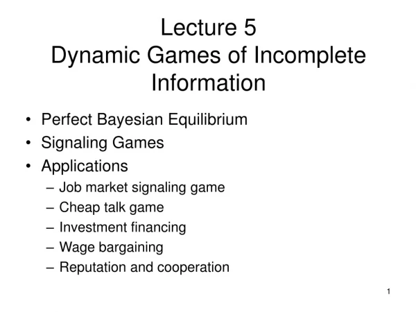
Lecture 5 Dynamic Games of Incomplete Information • Perfect Bayesian Equilibrium • Signaling Games • Applications • Job market signaling game • Cheap talk game • Investment financing • Wage bargaining • Reputation and cooperation
Dynamic Games of Incomplete Information : Example Player 2 1 R L’ R’ 1 3 M L 2 2 L R’ R’ L’ Player 1 M L’ R 2 1 0 0 0 2 0 1 Nash equilibrium : (L,L’), (R,R’) Subgame perfect Nash equilibrium : (L,L’), (R,R’) (no subgame) Perfect Bayesian equilibrium: (L,L’) and player 2’s belief: player 1 play L probability =1 (Whatever the belief, player 2 will play L’ )
Perfect Bayesian Equilibrium • Requirement 1(Belief): At each information set, the player with the move must have a belief about which node in the information set has been researched by the play of the game. For a nonsingleton information set, a belief is a probability distribution over the nodes in the information set; for a singleton information set, the player’s belief puts probability one on the single decision node
Perfect Bayesian Equilibrium (cont’) • Requirement 2 (Play based on belief): Given their beliefs, the players’ strategies must be sequentially rational. That is, at each information set the action taken by the player with the move (and the player’s subsequent strategy) must be optimal given the player belief at that information set and the other player’ subsequent strategies
Perfect Bayesian Equilibrium (cont’) • Definition: For a given equilibrium in a given extensive-form game, an information set is on the equilibrium if it will be reached with positive probability if the game is played according to the equilibrium strategies. And is off the equilibrium if it is certain not to be reached if the game is played according to the equilibrium strategies
Perfect Bayesian Equilibrium (cont’) • Requirement 3(Belief based on Bayes’ rule): At the information sets on the equilibrium path, beliefs are determined by Bayes’ rule and the players’ equilibrium strategies • Requirement 4(Reasonable belief): At the information sets off the equilibrium path, beliefs are determined by Bayes’ rule and the players’ equilibrium strategies where possible • Definition: A perfect Bayesian equilibrium consists of strategies and beliefs satisfying requirement 1 through 4
PBE: Example 1 1 R 1 3 L M 2 2 [p] [1-p] L’ R’ L’ R’ 2 1 0 0 0 2 0 1 If the play of the game reaches player 2’s nonsigleton information Given player 2’s belief, the expected payoff from playing R’ is UR’ =p.0+(1-p).1=1-p the expected payoff from playing L’ is UL’=p.1+(1-p).2=2-p UR’ < UL’for all p p=1 Subgame perfect Nash equilibrium : (L,L’) Subgame perfect Nash equilibrium : (R,R’) are ruled out
PBE: Example 2 1 A 2 0 0 D 2 • Information set is reached • (D, L, R’), p=1 : Nash equilibrium • (D, L, R’), p=1 : Subgame perfect Nash equilibrium • (D, L, R’), p=1 :Perfect Bayesian equilibrium • Information set is not reached • (A, L, L’),p=0 : Nash equilibrium • Given player 3’s belief p=0, player 3 play L; • Given player 3 play L’, player 2 play L • Given player 2, 3 play (L,L’), player 1 play A • (A, L, L’),p=0 : NOT subgame Nash equilibrium • Nash equilibrium of the only subgame is (L, R’) • (A, L, L’), p=0 : NOT Perfect Bayesian equilibrium • Player3’s belief p=0 conflicts with player 2 play L L R 3 [p] [1-p] L’ R’ L’ R’ 1 2 1 3 3 3 0 1 2 0 1 1
PBE: Example 3 • If player 1’s equilibrium strategy is A, requirement 4 may not determine 3’s belief from player 2 strategy (the player 3 ‘s information set is off equilibrium path) • 2. If player 2’s strategy is A’ then requirement 4 puts no restrictions on 3’s belief (the player 3 ‘s information set is off equilibrium path) • 3. If 2’s strategy is to play L with probability q1, R with probability q2, and A’ with probability 1-q1-q2, then requirement 4 dictates that 3’s belief be p=q1/(q1+q2) (the player 3 ‘s information set is on equilibrium path) A 1 D 2 A’ L R 3 [p] [1-p] L’ R’ L’ R’
Signaling Games • A signaling game is a dynamic game of incomplete information involving two players: a Sender (S) and a Receiver (R) • Timing of the game is as follows: • 1. Nature draws a type ti for the Sender from a set of feasible types T={t1,…,tI} according to a probability distribution p(ti), where p(ti)>0 for every i and p(t1)+…+p(tI)=1 • 2. The Sender observes ti and then chooses a message mj from a set of feasible M={m1,…,. mJ} • 3. The Receiver observes mj (but not ti) and then chooses an action akfrom a set of feasible actions A={a1,…,aK} • 4.Payoffs are given by US(ti,mj,ak) and UR(ti,mj,ak)
Signaling Games • A pure strategy for the Sender • is a function m(ti) specifying which message will be chosen for each type that nature might draw • A pure strategy for the Receiver • is a function a(mj) specifying which action will be chosen for each message that the Sender might send.
Signaling Games: Example Sender a1 a1 t1 m1 m2 a2 p a2 Receiver Nature Receiver a1 a1 1-p m1 m2 t2 a2 a2 Sender T={t1,t2}, M={m1,m2}, A={a1,a2}, and Prob(t1)=p
Signaling Games • Sender’s strategy • Strategy 1: m(t1)=m1 and m(t2)=m1(pooling strategy) • Strategy 2: m(t1)=m1 and m(t2)=m2(separating strategy) • Strategy 3: m(t1)=m2 and m(t2)=m1(separating strategy) • Strategy 4: m(t1)=m2 and m(t2)=m2(pooling strategy) • Receiver’s strategy • Strategy 1: a(m1)=a1 and a(m2)=a1(pooling strategy) • Strategy 2: a(m1)=a1 and a(m2)=a2(separating strategy) • Strategy 3: a(m1)=a2 and a(m2)=a1(separating strategy) • Strategy 4: a(m1)=a2 and a(m2)=a2(pooling strategy)
Signaling Games • Signaling Requirement 1: After observing any message mj from M, the Receiver must have a belief about which types could have sent mj. Denote this belief by the probability distribution μ(ti|mj), whereμ(ti|mj)>=0 for each tiin T, and
Signaling Games • Signaling Requirement 2R: For each mj in M, the Receiver’s action a*(mj) must maximize the Receiver’s expected utility, given the belief μ(ti|mj) about which types could have sent mj. That is a*(mj) solves • Signaling Requirement 2S: For each ti in T, the Sender’s message m*(ti) must maximize the Sender’s utility, given the receiver’s strategy a*(mj). That is m*(ti) solves
Signaling Games • Signaling Requirement 3: For each mjin M, If there exists tiin T such that m*(ti)=mj, then the Receiver’s belief at the information set corresponding to mj must follow from Bayes’ rule and the Sender’s strategy: • Definition: A pure-strategy perfect Bayesian equilibrium is a signaling game is a pair of strategies m*(ti)and a*(mj) and a belief μ(ti|mj) satisfying Signaling Requirements (1),(2R),(2S), and (3)
Signaling Games: Example Payoff of Receiver Sender 1,3 u u 2,1 Payoff of Sender [p] t1 [q] L R 4,0 d 0.5 d 0,0 Nature Receiver Receiver 2,4 u u 1,0 0.5 [1-q] [1-p] L R t2 d 0,1 d 1,2 Sender T={t1,t2},M={L,R},A={u,d}, and Prob(t1)=0.5
Signaling Games • Approach • Given the Sender’s strategy (m(t1), m(t2)), derive the receiver’s optimal strategy (a(L), a(R)) • Given receiver’s strategy, check whether the Sender’s strategy is optimal Type t1 Type t2 Signal L Signal R
Signaling Games The Sender’s strategy • Strategy 1: m(t1)=L and m(t2)=L (pooling) • The Receiver’s strategy: a(L)=u and a(R)=d, p=0.5, q<=2/3 (PBE) • If a(R)=u, then type t1Sender will deviate to play R • Condition for a(R)=d is q.0+(1-q).2>=q.1+(1-q).0 • Strategy 2: m(t1)=L and m(t2)=R (separating) • The Receiver’s strategy: p=1, q=0, a(L)=u and a(R)=d • No equilibrium (the type t2 Sender will deviate to play L ) • Strategy 3: m(t1)=R and m(t2)=L (separating) • The Receiver’s strategy: p=0,q=1, a(L)=u and a(R)=u, (PBE) • Strategy 4: m(t1)=R and m(t2)=R (pooling) • The Receiver’s strategy: q=0.5, a(R)=d , forall p, a(L)=u 0.5x0+0.5x2 (play d)>0.5x1+0.5x0 (play u) • No equilibrium (the type t1 Sender will deviate to play L)
Application 1: Corporate Investment and Capital Structure • An entrepreneur who has started a company but needs outside financing to undertake an attractive new project • The entrepreneur has private information about the profitability of the existing company • The payoff of the new project cannot be disentangled from the payoff of the existing company • The entrepreneur offers a potential investor an equity stake in the firm in exchange for the necessary financing
Application 1: Corporate Investment and Capital Structure (cont’) • Suppose the profit of the existing company cab be either high or low: π=H or L, where H>L>0 • The required investment is I and the payoff will be R, R>I(I+r), where r is the alternative rate of return
Application 1: Corporate Investment and Capital Structure (cont’) • Timing of the game • 1. Nature determines the profit of the existing company. The probability that π= L is p • 2. The entrepreneur learns π and then offers the potential investor an equity stake s, where 0<=s<=1 • 3. The investor observes s (but not π) and then decides either to accept or to reject the offer • 4. If the investor rejects the offer then the investor’s payoff is I(1+r) and the entrepreneur’s payoff is π. If the investor accepts s then the investor’s payoff is s(π+R) and the entrepreneur’s is (1-s) (π+R)
Application 1: Corporate Investment and Capital Structure (cont’) • Suppose that after receiving the offer s the investor believes that the probability that π= L is q • The investor will accept s if and only if • The entrepreneur will offer s if and only if • A pooling perfect Bayesian equilibrium (q=p) exists only if • (offer s no matter π is H or L ) • If p is close to zero • If p is close to one (1-s)(π+R)> π (always hold, cost of subsidization is small) (hold when profit outweighs cost of subsidization )
Application 1: Corporate Investment and Capital Structure (cont’) • Difficulty of a pooling equilibrium • The high-profit type must subsidize the low-profit type • If the subsidization is too expensive, high profit firm prefers to forego the new project
Application 1: Corporate Investment and Capital Structure (cont’) • A separating equilibrium always exists • The low-profit type offers • The investor accepts the offer • The high-profit type offers • The investor rejects the offer • While the new project is profitable, the high-profit type foregoes the investment • Implications • The investment is inefficiently low (only low-profit type) • The high-profit type cannot distinguish itself • Low-profit type will deviate to mimic high-profit type (the maximum equity)
Application 2: Sequential Bargaining under Asymmetric Information • Consider a firm and a union bargaining over wages • The firm’s profit, denoted by π, is uniformly distributed on [0, πH], but the true value of π is privately known by the firm • The bargaining game lasts at most two period • In the first period, the union makes an offer w1. If the firm accepts this offer then the game ends, otherwise proceeds to the second stage • The union’s payoff is w1, the firm’s payoff is π-w1 • In the second stage, the union makes a second offer, w2. • If the firm accepts the offer, then the union’s payoff is δw2, the firm’s payoff is δ(π-w2) • If the firm rejects the offer, then both players’ payoff are 0
Application 2: Sequential Bargaining under Asymmetric Information (cont’) • Assume the union offers w1 in the first period and the firm expects the union to offer w2 in the second period. • The firm prefers accepting w1 to accepting w2 if π-w1>0 (individual rationality) and π-w1>δ(π-w2) (incentive compatibility) • If the firm reject w1, the union’s adjusted belief at the information set is that π is uniformly distributed on [0, π1 *] • The union’s optimal second-period offer w2* is π1*/2 Solve (the firm accepts w2) (the firm rejects w2)
Application 2: Sequential Bargaining under Asymmetric Information (cont’) • The union first’s period wage offer should be chosen to solve If π1*=w1 then (contradiction) the firm rejects both w1and w2 In the first period the firm accepts w1 In the second period the firm accepts w2
Application 2: Sequential Bargaining under Asymmetric Information (cont’) • The unique perfect Bayesian equilibrium • The union’s first-period wage offer is w1* • If the firm’s profit, π, exceeds π1*, then the firm accepts w1*;otherwise the firm reject w1* • The union’s second-period wage offer (conditional on w1* is rejected) is w2* • If the firm’s profit π, exceeds w2* then the firm accepts the offer; otherwise, it rejects it • Implication • low-profit firms tolerate a one-period strike in order to convince the union that they are low-profit and so induce the union to offer a lower second-period wage • Firms with very low profits, however, find even the lower second-period intolerably high and so reject it too
Application 3: Job-Market Signaling • Timing of the game • 1. Nature determines a worker’s productive abilityη, which can be either high (H) or low (L). The probability that η=H isq • 2. The worker learns his or her ability and then chooses a level of education, e>=0 • 3. Two firms observe the work’s education (but not the worker’s ability) and then simultaneously make wage offers to the worker • 4. The worker accepts the higher of the two wage offers, flipping a coin in case of a tie. Let w denote the worker accepts
Application 3: Job-Market Signaling (cont’) • Spence’s model (1973) • Education cost: c(η,e) is the cost to a work with ability ηof obtaining education e • Output: y(η,e) is the output of a worker with ability ηof obtaining education e • The worker’s payoff: w-c(η,e) • The firm’s payoff: y(η,e)-w
Application 3: Job-Market Signaling (cont’) • Critical assumption: low-ability worker find signaling more costly than do high-ability workers. • The marginal cost of education is higher for low-ability than for high-ability worker: for every e, ce(L,e)>ce(H,e) IL IH wL wH w1 e1 e2
Application 3: Job-Market Signaling (cont’) • Competition among firms will drive expected profits to zero • The market would offer a wage equal to the expected output of a worker with education e, given the market’s belief about the worker’s ability after observing e • where is the market’s assessment of the probability that the worker’s ability is H • w(e)=y(η,e)
Application 3: Job-Market Signaling (cont’) • A worker with ability ηchoose e to solve Indifference curves for abilityη UA w UA>UB>UC UB UC y(η,e) w*(η) e e*(η)
Application 3: Job-Market Signaling (cont’) Scenario 1 w IH IL y(H,e) w*(H) y(L,e) w*(L) e e*(L) Too expensive for the low-ability worker to acquire e*(H)
Application 3: Job-Market Signaling (cont’) Scenario 2 IH w IL y(H,e) w*(H) y(L,e) w*(L) e e*(L) e*(H) The low-ability worker could masquerade (伪装) as a high-ability worker
Application 3: Job-Market Signaling (cont’) Pooling perfect Bayesian equilibria qy(H,e)+(1-q)y(L,e) y(H,e) IH w IL qy(H,e)+(1-q)y(L,e) we’ y(L,e) wp w*(L) e e*(L) ep e’
Application 3: Job-Market Signaling (cont’) Separating perfect Bayesian equilibria IH w IL y(H,e) Wes* wes y(L,e) w*(H) w*(L) es es* e e*(L) e*(H)
Application 4: Cheap-Talk Games • The Sender’s messages are just talk – costless, nonbinding, nonverifiable claims • Cheap talk can or cannot be informative • In Spence’s signaling game, cheap talk cannot be informative. All workers prefer higher wage. Therefore, a worker who simply announced “my ability is high” would not be believed • Necessary conditions for cheap talk to be informative • 1. Different Sender-types have different preferences over the Receiver’s actions • 2. The Receiver prefer different actions depending on the Sender’s type • 3. The receiver’s preferences over actions not be completely opposed to the Sender’s
Application 4: Cheap-Talk Games (cont’) • Timing of the simplest cheap-talk • identical to the timing of the simplest signaling game; only payoffs differ • 1. Nature draws a type tifor the Sender from a set of feasible types T={t1,…,tI} according to a probability distribution p(ti), where p(ti)>0 for every i and p(t1)+…+p(tI)=1 • 2. The Sender observes ti and then chooses a message mj from a set of feasible messages M={m1,…mJ} • 3.The Receiver observes mj(but not ti) and then chooses an action ak from a set of feasible actions A={a1,…,ak} • 4. Payoffs are given by US(ti,ak) and UR(ti,ak)
Application 4: Cheap-Talk Games (cont’) • A pooling equilibrium • Always exists • The Sender’s strategy: Messages have no direct effect on the Sender’s payoff. If the Receiver will ignore all messages then pooling is the best response for the Sender • The Receiver’s strategy: Messages have no direct effect on the Receiver’s payoff. If the Sender is pooling,then the best response for the Receiver’s optimal action is to ignore all message • Let a* denote the Receiver’s optimal action in a pooling equilibrium. That is a* solves
Application 4: Cheap-Talk Games (cont’) • A separating equilibrium Sender’s payoff Receiver’spayoff tL tH Separating equilibrium : Sender’s strategy:[m(tL)=tL,m(tH)=tH] Receiver’s beliefs:μ(tL|tL)=1, μ(tL|tH)=0 Receiver’s strategy:a(tL)=aL, a(tH)=aH aL aH The Receiver prefers the low action (aL) when the Sender’s type is low (tL) and the high action (aH) when the type is high (tH) If x>z and y>w, then both types would like the Receiver to believe that t=tL If z>x and y>w, tL(tH) would like the Receiver to believe that t=tH(t=tL) Separating equilibrium exists if and only if x>= zand w>= y
Application 4: Cheap-Talk Games (cont’) • Crawford and Sobel’s model (1982) • The type, message, and action spaces are continuous • The Sender’s type is uniformly distributed between zero and one (T=[0,1] ); the message space is the type space (M=T); and the action space is the interval from zero to one (A=[0,1]) • The Receiver’s payoff function is UR(t,a)=-(a-t)2 and the Sender’s is US(t,a)=-[a-(t+b)]2 • When the Sender’s type is t, the receiver’s optimal action is a=tbut the Sender’s optimal action is a=t+b • The parameter b>0 measures the similarity of the players’ preference • Different Sender-types have different preferences over the Receiver’s actions (higher types prefer higher actions) • When b is closer to zero, the players’ interests are more closely aligned
Application 4: Cheap-Talk Games (cont’) • Partially pooling equilibrium • The type space is divided into the n intervals [0,x1), [x1,x2),…,[xn-1,1]; all types in a given interval send the same message, but types in different intervals send different message • n=2 : the type space is divided to [0,x1) and [x1,1] • the Receiver’s optimal action will be x1/2 after receiving a message from types in [0,x1] • the Receiver’s optimal action will be (x1+1)/2 after receiving a message from types in [x1,1]
Application 4: Cheap-Talk Games (cont’) Two steps (n=2) X1/2 (X1+1)/2 t+b a=0 a=1 [X1/2+ (X1+1)/2]/2 US (t,a) • Atype t Sender will prefer to x1/2 if t+b=<[x1/2+(x1+1)/2]/2 • A type t Sender will prefer to (x1+1)/2 if t+b>=[x1/2+(x1+1)/2]/2 • Equilibrium condition: type x1 is indifferent in [0,x1) or [x1,1] (x1+b)- x1/2= (x1+1)/2-(x1+b) x1+b=[x1/2+ (x1+1)/2]/2 x1=1/2-2b , where b<1/4
Application 4: Cheap-Talk Games (cont’) • N steps [0,x1), [x1,x2),…,[xn-1,1] • the Receiver’s optimal action will be(xk+xk-1)/2 after receiving a message from types in [xk-1,xk) • the Receiver’s optimal action will be(xk+1+xk)/2 after receiving a message from types in [xk,xk+1) • A type xk Sender optimal actions is xk+b • To make the boundary type xk indifferent between [xk-1,xk) and [xk,xk+1) (xk+1+xk)/2 – (xk+b) = (xk+b) - (xk+xk-1)/2 xk+1-xk= xk-xk-1+4b
Application 4: Cheap-Talk Games (cont’) • If the first step is if length d and nth step end exactly at t=1 d+(d+4b)+…+[d+(n-1)4b]=1 nd+n(n-1)2b=1 Implication: More communication can occur through cheap talk when the players’ preferences are more closely
Application 5: Reputation in the Finitely Repeated Prisoners’ Dilemma • Theoretical result: If a stage game has a unique Nash equilibrium, the any finitely repeated game based on this stage game has a unique subgame Nash equilibrium: the Nash equilibrium of the stage game is played in every stage, after every history • Complete information on the playoff functions • Experimental evidence: Cooperation occurs frequently during finitely repeated Prisoners’ Dilemmas, especially in stages that are not too close to the end • Explanation of the evidence : KMRW’s reputation model (1982) • Asymmetric information on the strategy
Application 5: Reputation in the Finitely Repeated Prisoners’ Dilemma • Tit-for-Tat strategy • begins the repeated game by cooperating and thereafter mimics the opponent’s previous play • Was the winning entry in Axelrod’s prisoners’ dilemma tournament • KMRW’s reputation model • Assume the player has private information about his or her feasible strategies • With probability p the a player can play only Tit-for-Tat strategy, while 1-p that can play any of the strategies available in the complete-information repeated game (including Tit-for-Tat) (rational)
Application 5: Reputation in the Finitely Repeated Prisoners’ Dilemma • The timing of the game • 1. Nature draws a type for the Row player: With probability p, Row has only the Tit-for-Tat strategy available; with probability 1-p, Row can play any strategy. Row learns his or her type, but Column does not learn Row’s type • 2. Row and Column play the Prisoners’ Dilemma. The players’ choices in the stage game become common knowledge • 3. Row and Column play the Prisoners’ Dilemma for a second and last time • 4. Payoffs are received. The payoffs to the Row and to Column are the sums of their stage-game payoffs