Download

1 / 91
910 likes | 932 Views
Investigate the best static tree structure with known frequencies; analyze splay tree optimization for efficient access sequences.

E N D
Motivation • Assume you know the frequencies p1, p2 , …. • What is the best static tree ? • You can find it in O(nlog(n)) time (homework)
0.1 0.26 0.2 0.1 Approximation (Mehlhorn) .04 0.2 0.1 0.26 0.1 0.2 0.1
Approximation (Mehlhorn) .04 0.2 0.1 0.26 0.1 0.2 0.1 0.1 0.26 0.2 0.1
.04 0.2 0.1 0.26 0.1 0.2 0.1 0.26 0.2 0.1
.04 0.2 0.1 0.26 0.1 0.2 0.1 0.26 0.2 0.1
.04 0.2 0.1 0.26 0.1 0.2 0.1 0.26 0.2 0.1
.04 0.2 0.1 0.26 0.1 0.2 0.1 0.26 0.2 0.1
.04 0.2 0.1 0.26 0.1 0.2 0.1 0.26 0.2 0.1
.04 0.2 0.1 0.26 0.1 0.2 0.1 0.26 0.2 0.1
.04 0.2 0.1 0.26 0.1 0.2 0.1 0.26 0.2 0.1
.04 0.2 0.1 0.26 0.1 0.2 0.1 0.26 0.2 0.1
.04 0.2 0.1 0.26 0.1 0.2 0.1 0.26 0.2 0.1
.04 0.2 0.1 0.26 0.1 0.2 0.1 0.26 0.2 0.1
.04 0.2 0.1 0.26 0.1 0.2 0.1 0.26 0.2 0.1
.04 0.2 0.1 0.26 0.1 0.2 0.1 0.26 0.2 0.1
.04 0.2 0.1 0.26 0.1 0.2 0.1 0.26 0.2 0.1
Analysis .04 0.2 0.1 0.26 0.1 0.2 0.1 0.26 0.2 0.1 An internal node at level i corresponds to an interval of length 1/2i The sum of the weights of the pieces that correspond to an internal node is no larger than the length of the corresponding interval
Analysis .04 0.2 0.1 0.26 0.1 0.2 0.1 0.26 0.2 0.1
Main idea • Try to arrange so frequently used items are near the root • We shall assume that there is an item in every node including internal nodes. We can change this assumption so that items are at the leaves.
First attempt Move the accessed item to the root by doing rotations y x <===> x C A y B C A B
e e e d F d F d F E E c a E c A c b a A b A B C D B b a D C D B C Move to root (example)
Move to root (analysis) There are arbitrary long access sequences such that the time per access is Ω(n) ! Homework ?
z y D C x A B Splaying Does rotations bottom up on the access path, but rotations are done in pairs in a way that depends on the structure of the path. A splay step: (1) zig - zig x ==> A y B z C D
Splaying (cont) (2) zig - zag z x ==> y D y z A B C D x A B C (3) zig y x ==> x C A y B C A B
i i ==> ==> h h J J g I g I f H f H A e A a d G d e a b F G B B b c F E c E C D D C Splaying (example) i h J g I f H A e d G c B b C a D E F
i ==> ==> a h J h a I f g i A d e f H I J g b F G e B A d H c F G E b B C D c E C D Splaying (example cont) i h J g I f H A a d e b F G B c E C D
Splaying (analysis) Assume each item i has a positive weight w(i) which is arbitrary but fixed. Define the sizes(x) of a node x in the tree as the sum of the weights of the items in its subtree. The rank of x: r(x) = log2(s(x)) Measure the splay time by the number of rotations
Access lemma The amortized time to splay a node x in a tree with root t is at most 3(r(t) - r(x)) + 1 = O(log(s(t)/s(x))) Potential used: The sum of the ranks of the nodes. This has many consequences:
Balance theorem Balance Theorem: Accessing m items in an n node splay tree takes O((m+n) log n) Proof:
Proof of the access lemma The amortized time to splay a node x in a tree with root t is at most 3(r(t) - r(x)) + 1 = O(log(s(t)/s(x))) proof. Consider a splay step. Let s and s’, r and r’ denote the size and the rank function just before and just after the step, respectively. We show that the amortized time of a zig step is at most 3(r’(x) - r(x)) + 1, and that the amortized time of a zig-zig or azig-zag step is at most 3(r’(x)-r(x)) The lemma then follows by summing up the cost of all splay steps
Proof of the access lemma (cont) (3) zig y x ==> x C A y B C A B amortized time(zig) = 1 + = 1 + r’(x) + r’(y) - r(x) - r(y) 1 + r’(x) - r(x) 1 + 3(r’(x) - r(x))
z y D C x A B Proof of the access lemma (cont) (1) zig - zig x ==> A y B z C D amortized time(zig-zig) = 2 + = 2 + r’(x) + r’(y) + r’(z) - r(x) - r(y) - r(z) = 2 + r’(y) + r’(z) - r(x) - r(y) 2 + r’(x) + r’(z) - 2r(x) 2r’(x) - r(x) - r’(z) + r’(x) + r’(z) - 2r(x) = 3(r’(x) - r(x)) 2 -(log(p) + log(q)) = log(1/p) + log(1/q) = log(s’(x)/s(x)) + log(s’(x)/s(z))= r’(x)-r(x) + r’(x)-r(z)
Proof of the access lemma (cont) (2) zig - zag z x ==> y D y z A B C D x A B C Similar. (do at home)
Intuition 9 8 7 6 5 4 3 2 1
Intuition 9 9 8 8 7 7 6 6 5 5 = 0 4 4 3 1 2 2 3 1
9 9 8 8 7 7 6 6 5 1 4 4 5 = log(5) – log(3) + log(1) – log(5) = -log(3) 2 1 3 2 3
9 9 8 8 1 7 6 6 7 4 5 1 2 4 3 5 = log(7) – log(5) + log(1) – log(7) = -log(5) 2 3
1 9 8 9 8 6 7 1 4 6 5 2 7 4 3 5 2 3 = log(9) – log(7) + log(1) – log(9) = -log(7)
Static optimality theorem: If every item is accessed at least once then the total access time is O(m + q(i) log (m/q(i)) ) n i=1 Static optimality theorem For any item i let q(i) be the total number of time i is accessed Optimal average access time up to a constant factor.
Static finger theorem: Let f be an arbitrary fixed item, the total access time is O(nlog(n) + m + log(|ij-f| + 1)) m j=1 Static finger theorem Suppose all items are numbered from 1 to n in symmetric order. Let the sequence of accessed items be i1,i2,....,im Splay trees support access within the vicinity of any fixed finger as good as finger search trees.
Working set theorem Let t(j), j=1,…,m, denote the # of different items accessed since the last access to item j or since the beginning of the sequence. Working set theorem: The total access time is Proof:
Application: Data Compression via Splay Trees Suppose we want to compress text over some alphabet Prepare a binary tree containing the items of at its leaves. • To encode a symbol x: • Traverse the path from the root to x spitting 0 when you go left and 1 when you go right. • Splay at the parent of x and use the new tree to encode the next symbol
a b a b c d e f g h c d e f g h Compression via splay trees (example) aabg... 000
a b a b c d e f g h c d e f g h Compression via splay trees (example) aabg... 000 0
a b c d e f g h Compression via splay trees (example) a b c d e f g h aabg... 0000 10
a b c d e f g h Compression via splay trees (example) a b c d e f g h aabg... 0000 10 1110
Decoding Symmetric. The decoder and the encoder must agree on the initial tree.