Download
1 / 23
230 likes | 246 Views
This workshop discusses the analysis of frame delay distribution in 802.11 using signal flow graphs. It covers scenarios, DCF in IEEE 802.11, analytical modeling, VoIP capacity calculation, and more.

E N D
19th FFV Workshop Frame Delay Distribution Analysis of 802.11 Using Signal Flow Graphs Ralf Jennen Communication Networks Research Group RWTH Aachen University, Faculty 6, Germany FFV Workshop, 11.03.2011
Outline • Scenarios • Distributed Coordination Function (DCF) in IEEE 802.11 • Modelling of IEEE 802.11a DCF • Development of an analytical model • From a saturated to a non-saturated model • VoIP capacity calculation • Conclusion & Outlook
WLAN Scenarios • Best Case Scenario • All STAs with MC1 • Worst Case Scenario • All STAs with MC8 • Mixed Scenarios • Tagged MC1 / other STAs MC8 • Tagged MC8/other STAs MC1 Tagged Station MC8 = BPSK 1/2 Tagged AP … MC1 = 64-QAM 3/4 … α r1 … AP r8 STA 02 Terminal Buffer STA 01 STA N AP = Access PointMC = Modulation and Coding STA = Station
Readyto Send/Clear to Send (RTS/CTS) SIFS SIFS SIFS CTSTimeout DIFS DIFS DIFS Source/Tagged RTS Backoff RTS Data Destination/AP CTS ACK Other Station RTS Backoff Duration of a collision Successful transmission TSUCC TCOLL ACK = AcknowledgmentCTS = Clear to SendDCF = Distributed Coordination FunctionDIFS = DCF Interframce SpaceEIFS = Extended Interframe SpaceNAV = Network Allocation VectorRTS = Ready to SendSIFS = Short Interframe Space SLOT SIFS DIFS TimeoutA Station A/Tagged RTS NAV (RTS) EIFS Station B/Tagged Station C RTS Station D CTS RTS Duration of other stations‘ collisions TCOLL2 TCOLL1
Development of the Analytical Model SaturatedModel RTS/CTSBasic access Signal Flow Graph p τ Frame delay distribution for STAs WLANScenario Non-saturatedModel Link Adaptation Signal Flow Graph Frame delay distribution for STAs pi, τi, λ Queues WLANScenario pi, τi EmptyProbability WLANScenario VoIP traffic Up- andDownlink Morkov Modulated Poisson Process Signal Flow Graph Frame delay distribution for STAs and AP VoIP delay Queuing delay and service time Frame delaydistribution VoIP QoSRequirements VoIP capacity MMAP/G/1Queuing Model AP = Access pointG = General service time distribution i = per MCS and/or per STA or AP λ = Arrival rateMCS = Modulation and coding schemeMMAP = Marked Markov arrival process p= Collision probabilityQoS = Quality of ServiceSTA = Stationτ = Probability that station transmits in a given slot VoIP = Voice over IP
Saturated Conditions: Collision Probability Columns: Backoff Counter Signal Flow Graph for Backoff Stage 1/(W0+1) 1/(W0+1) 1/(W0+1) 0,0 0,1 0,W0 Related Work by: Bianchi, Duffy, Malone, Leith, Huang … 1-p p … 1/(W1+1) 1/(W1+1) 1/(W1+1) 1,0 1,1 1,W1 … 1-p p Rows: Backoff Stages … … 1/(Wm+1) 1/(Wm+1) 1/(Wm+1) m,0 m,1 m,Wm … 1-p p B(i,j) = Backoff state (stage/counter) k = Maximum of retransmissionsm = Window is doubled m-timesWi= Contention window at stage ip= Collision probability … … 1/(Wm+1) 1/(Wm+1) 1/(Wm+1) k,0 k,1 k,Wm …
Signal Flow Graph of one Backoff Stage 0 Backoff Slots pi Bi-1 Bi Idle Slot pidle IW1 pidle 1 Backoff Slot I11 Collision pcoll pcoll LW1 LW2 Bi = Backoff state for stage iL = Listening I =Idle slotC = CollisionS = Successful transmisssion pi= Backoff counter probabilityW = Contention Windowz = Delay operatorlc= Duration of a collisionl= Duration of a transmissionGi(z) = Delay Generation Function pi L11 C11 E1 psucc psucc Success S11 2 Backoff Slots pidle pidle I21 I22 pcoll pcoll pi L21 C21 L22 C22 E2 psucc psucc S21 S22 W Backoff Slots … … … pidle IWW pi pcoll Signal Flow Graph can be written as a Delay Generation Function: … EW CW1 LWW CWW psucc SW1 SWW
Signal Flow Graph of one Backoff Stage 0 Backoff Slots pi Bi-1 Bi Idle Slot pidle IW1 pidle 1 Backoff Slot I11 Collision pcoll pcoll LW1 LW2 Bi = Backoff state for stage iL = Listening I =Idle slotC = CollisionS = Successful transmisssion pi= Backoff counter probabilityW = Contention Windowz = Delay operatorlc= Duration of a collisionl= Duration of a transmissionGi(z) = Delay Generation Function pi L11 C11 E1 psucc psucc Success S11 2 Backoff Slots pidle pidle I21 I22 pcoll pcoll pi L21 C21 L22 C22 E2 psucc psucc S21 S22 W Backoff Slots I … … … pidle IWW C1 For each modulation and coding scheme i an own C and S state with corresponding delays , must be added pi pcoll … C2 EW CW1 LWW CWW LW EW psucc S1 SW1 SWW S2
Signal Flow Graph oftheUplink Frame Delay forSaturated Traffic T B0 Bk Bm E … … … Bk-1 Bi-1 Consider previous transmission F Bi = Backoff state for stage iE = Error stateF = Final stateGi(z) = Delay Generation Function for stage ik = Maximum of retransmissionsm = Backoff window is doubled m-timesp= Collision probabilityT = Transmit statez = Delay operator
From Saturated to Non-saturated Conditions: Collision Probability Columns: Backoff Counter 1/(W0+1) 1/(W0+1) 1/(W0+1) 0,0 0,1 0,W0 Related Work by: Bianchi, Duffy, Malone, Leith, Huang … 1-p p … 1/(W1+1) 1/(W1+1) 1/(W1+1) 1,0 1,1 1,W1 … 1-p p Rows: Backoff Stages … … 1/(Wm+1) 1/(Wm+1) 1/(Wm+1) m,0 m,1 m,Wm … 1-p p B(i,j) = Backoff state (stage/counter) k = Maximum of retransmissionsm = Window is doubled m-timesWi= Contention window at stage ip= Collision probability … … 1/(Wm+1) 1/(Wm+1) 1/(Wm+1) k,0 k,1 k,Wm …
Non-Saturated Conditions:Collision, Idle and Empty Probability 1/(W0+1) 1/(W0+1) 1/(W0+1) Backoff withoutframe (1-q0e)r1pidle(1-p)+(1-r2)(1-pidle) 0,0e 0,1e 0,W0e 1-r3 1-r3 (1-r1)pidle … r3 r3 r2(1-pidle) + q0er1pidle(1-p) … 1/(W0+1) 1/(W0+1) 1/(W0+1) 1/(W0+1) 1/(W0+1) (1-p)(1-q0) 0,0 0,1 0,W0 Related Work by: Bianchi, Duffy, Malone, Leith, Huang … (1-p)q0 r1ppidle p … (1-p)(1-q1) 1/(W1+1) 1/(W1+1) 1/(W1+1) 1,0 1,1 1,W1 … (1-p)q1 Stage dependentempty probability p … … (1-p)(1-qm) 1/(Wm+1) 1/(Wm+1) 1/(Wm+1) m,0 m,1 m,Wm … (1-p)qm B(i,j) = Backoff state k = Maximum of retransmissionsm = Window is doubled m-timesWi= Contention Window at stage ipidle= Idle Probability 1-qi= Queue empty probabilityri= Arrival probabilities p … … 1-qm 1/(Wm+1) 1/(Wm+1) 1/(Wm+1) k,0 k,1 k,Wm qm …
Non-Saturated Conditions:Previous Transmission Successful 1/(W0+1) 1/(W0+1) 1/(W0+1) (1-q0e)r1pidle(1-p)+(1-r2)(1-pidle) 0,0e 0,1e 0,W0e 1-r 1-r (1-r1)pidle … r r r2(1-pidle) + q0er1pidle(1-p) … Special statewithout collisions 1/(W0+1) 1/(W0+1) 1/(W0+1) 1/(W0+1) 1/(W0+1) 1/(W0+1) (1-p)(1-q0) 0,0f q0f 0,0 0,1 0,W0 1-q0f Related Work by: Bianchi, Duffy, Malone, Leith, Huang … (1-p)q0 r1ppidle p … (1-p)(1-q1) 1/(W1+1) 1/(W1+1) 1/(W1+1) 1,0 1,1 1,W1 … (1-p)q1 p … … (1-p)(1-qm) 1/(Wm+1) 1/(Wm+1) 1/(Wm+1) m,0 m,1 m,Wm … (1-p)qm B(i,j) = Backoff state k = Maximum of retransmissionsm = Window is doubled m-timesWi= Contention window at stage ipidle= Idle probability 1-qi= Buffer empty probability r = Arrival probability p … … 1-qm 1/(Wm+1) 1/(Wm+1) 1/(Wm+1) k,0 k,1 k,Wm (1-p)qm … pqm
Signal Flow Graph of the Frame Delay forNon-saturated Downlink Traffic T B0 B1 E T B0 F Bk E Bm … … … Bk-1 Bi-1 F Bi = Backoff state for stage iE = Error stateF = Final stateGi(z) = Delay Generation Function for stage ik = Maximum of retransmissionsm = Backoff window is doubled m-timesp= Collision probabilityT = Transmit statez = Delay operator
Signal Flow Graph of the Frame Delay forNon-saturated Downlink Traffic MMAP(i)/G(i)/1 with i different classes W T B0 B1 E … F Related Work by: He, Takine, Göbbels S SA SB SC Bi = Backoff state for stage iE = Error stateF = Final stateG(i) = General service time distributionGi(z) = Delay generation function for stage iGQ(z) = Delay generation function for queuingi = Number of modulation and coding schemes k = Maximum of retransmissions m = Backoff window is doubled m-timesMMAP = Marked Markov arrival processp= Collision probabilitype = System empty probabilityS = Serving stateT = Transmit stateW = Waiting state
Three Possible Arrivals:1. During Countdown 1/(W0+1) 1/(W0+1) 1/(W0+1) Duringcountdown (1-q0e)r1pidle(1-p)+(1-r2)(1-pidle) 0,0e 0,1e 0,W0e 1-r3 1-r3 (1-r1)pidle … r3 r3 r2(1-pidle) + q0er1pidle(1-p) … 1/(W0+1) 1/(W0+1) 1/(W0+1) 1/(W0+1) 1/(W0+1) (1-p)(1-q0) Continue withbackoff stage 0 0,0 0,1 0,W0 … (1-p)q0 r1ppidle p … (1-p)(1-q1) 1/(W1+1) 1/(W1+1) 1/(W1+1) 1,0 1,1 1,W1 … (1-p)q1 p … … (1-p)(1-qm) 1/(Wm+1) 1/(Wm+1) 1/(Wm+1) m,0 m,1 m,Wm … (1-p)qm B(i,j) = Backoff state k = Maximum of retransmissionsm = Window is doubled m-timesWi= Contention window at stage ipidle= Idle probability 1-qi= Buffer empty probability r = Arrival probability p … … 1-qm 1/(Wm+1) 1/(Wm+1) 1/(Wm+1) k,0 k,1 k,Wm qm …
Signal Flow Graph of the Frame Delay forNon-saturated Downlink Traffic W T B0 B1 E … F S SA Coefficients of GA arefunctions of G0 SB SC Bi = Backoff state for stage iE = Error stateF = Final stateG(i) = General service time distributionGi(z) = Delay generation function for stage iGQ(z) = Delay generation function for queuingi = Number of modulation and coding schemes k = Maximum of retransmissions m = Backoff window is doubled m-timesMMAP = Marked Markov arrival processp= Collision probabilitype = System empty probabilityS = Serving stateT = Transmit stateW = Waiting state
Three Possible Arrivals:2. Medium Idle in B(0,0)e 1/(W0+1) 1/(W0+1) 1/(W0+1) In B(0,0)e andmedium idle (1-q0e)r1pidle(1-p)+(1-r2)(1-pidle) 0,0e 0,1e 0,W0e 1-r3 1-r3 (1-r1)pidle … r3 r3 r2(1-pidle) + q0er1pidle(1-p) … 1/(W0+1) 1/(W0+1) 1/(W0+1) 1/(W0+1) 1/(W0+1) (1-p)(1-q0) Continue with orwithout frame 0,0 0,1 0,W0 … (1-p)q0 r1ppidle p … (1-p)(1-q1) 1/(W1+1) 1/(W1+1) 1/(W1+1) 1,0 1,1 1,W1 … (1-p)q1 p … … (1-p)(1-qm) 1/(Wm+1) 1/(Wm+1) 1/(Wm+1) m,0 m,1 m,Wm … (1-p)qm B(i,j) = Backoff state k = Maximum of retransmissionsm = Window is doubled m-timesWi= Contention window at stage ipidle= Idle probability 1-qi= Buffer empty probability r = Arrival probability p … … 1-qm 1/(Wm+1) 1/(Wm+1) 1/(Wm+1) k,0 k,1 k,Wm qm …
Signal Flow Graph of the Frame Delay forNon-saturated Downlink Traffic W T B0 B1 E … F S SA No additional delay SB SC Bi = Backoff state for stage iE = Error stateF = Final stateG(i) = General service time distributionGi(z) = Delay generation function for stage iGQ(z) = Delay generation function for queuingi = Number of modulation and coding schemes k = Maximum of retransmissions m = Backoff window is doubled m-timesMMAP = Marked Markov arrival processp= Collision probabilitype = System empty probabilityS = Serving stateT = Transmit stateW = Waiting state
Three Possible Arrivals:3. Medium Busy in B(0,0)e 1/(W0+1) 1/(W0+1) 1/(W0+1) In B(0,0)e andmedium busy (1-q0e)r1pidle(1-p)+(1-r2)(1-pidle) 0,0e 0,1e 0,W0e 1-r3 1-r3 (1-r1)pidle … r3 r3 r2(1-pidle) + q0er1pidle(1-p) … 1/(W0+1) 1/(W0+1) 1/(W0+1) 1/(W0+1) 1/(W0+1) (1-p)(1-q0) Continue withbackoff stage 0 0,0 0,1 0,W0 … (1-p)q0 r1ppidle p … (1-p)(1-q1) 1/(W1+1) 1/(W1+1) 1/(W1+1) 1,0 1,1 1,W1 … (1-p)q1 p … … (1-p)(1-qm) 1/(Wm+1) 1/(Wm+1) 1/(Wm+1) m,0 m,1 m,Wm … (1-p)qm B(i,j) = Backoff state k = Maximum of retransmissionsm = Window is doubled m-timesWi= Contention window at stage ipidle= Idle probability 1-qi= Buffer empty probability r = Arrival probability p … … 1-qm 1/(Wm+1) 1/(Wm+1) 1/(Wm+1) k,0 k,1 k,Wm qm …
Signal Flow Graph of the Frame Delay forNon-saturated Downlink Traffic W T B0 B1 E … F S SA SB Coefficients of GC dependon GSUCC and GCOLL SC Bi = Backoff state for stage iE = Error stateF = Final stateG(i) = General service time distributionGi(z) = Delay generation function for stage iGQ(z) = Delay generation function for queuingi = Number of modulation and coding schemes k = Maximum of retransmissions m = Backoff window is doubled m-timesMMAP = Marked Markov arrival processp= Collision probabilitype = System empty probabilityS = Serving stateT = Transmit stateW = Waiting state
VoIP Capacity Example • Satisfied User Criteria • Meanopinion score • Satisfiediflessthen 2% ofthepackets do not arrivearrivesuccessfullyattheradioreceiverwithin 50ms = 5555 SLOT • QoSRequirements • Frame error rate • End to end delay • Jitter • ITU G.711packet size=120 Byte packet rate=1/10 msactive=352 msinactive=650 ms Related Work by: Tobagi, Hole,Chen, Garg, Kappes • Next steps: • Frame delay + waiting time • Find N that fulfils the satisfied user criteria
Conclusion & Outlook Conclusion • Development of the Analytical Model • Scenarios and DCF Overview • Signal Flow Graph Model of 802.11 DCF • Extension of the Signal Flow Graph • Frame delay for non-saturated conditions • VoIP capacity calculation Outlook • VoIP capacity for multiple scenarios • Interference model, additional packet loss • Validated results by event driven simulation
Thank you for your attention ! Ralf Jennen jen@comnets.rwth-aachen.de The research leading to these results has received funding from the European Union's Seventh Framework Programme ([FP7/2007-2013] ) under grant agreement number ICT-213311