Poisson Process and Probability Distributions
80 likes | 162 Views
Explore the Poisson distribution, inter-arrival times, and random arrivals in the context of probability theory. From arrival rates to independent random variables, delve into the intricacies and applications of this statistical model.

Poisson Process and Probability Distributions
E N D
Presentation Transcript
CIS 2033 based onDekking et al. A Modern Introduction to Probability and Statistics. 2007 Instructor Longin Jan Latecki C12: The Poisson process
12.2 – Poisson Distribution Definition: A discrete RV X has a Poisson distribution with parameter µ, where µ > 0 if its probability mass function is given by for k = 0,1,2…, where µ is the expected number of rare events occurring in time interval [0, t], which is fixed for X. We can express µ =t λ, where t is the length of the interval, e.g., number of minutes. Hence λ = µ / t= number of events per time unite = probability of success. λ is also called the intensity or frequency of the Poisson process. We denote this distribution: Pois(µ) = Pois(tλ). Expectation E[X] = µ = tλand variance Var(X) = µ = tλ
Let X1, X2, … be arrival times such that the probability of k arrivals in a given time interval [0, t] has a Poisson distribution Pois(tλ): The differences Ti = Xi – Xi-1 are called inter-arrival times or wait times. The inter-arrival times T1=X1, T2=X2 – X1, T3=X3 – X2 … are independent RVs, each with an Exp(λ) distribution. Hence expected inter-arrival time is E(Ti) =1/λ. Since for Poisson λ = µ / t= (number of events) / (time unite) = probability of success, we have for the exponential distribution E(Ti) =1/λ = t / µ = (time unite) / (number of events) = wait time
Let X1, X2, … be arrival times such that the probability of k arrivals in a given time interval [0, t] has a Poisson distribution Pois(λt): Each arrival time Xi, is a random variable with Gam(i, λ) distribution for α=i : We also observe that Gam(1, λ) = Exp(λ):
12.2 –Random arrivals • Example: Telephone calls arrival times • Calls arrive at random times, X1, X2, X3… • Homegeneity aka weak stationarity: is the rate lambda at which arrivals occur in constant over time: in a subinterval of length u the expectation of the number of telephone calls is λu. • Independence: The number of arrivals in disjoint time intervals are independent random variables. • N(I) = total number of calls in an interval I • Nt=N([0,t]) • E[Nt] = t λ • Divide Interval [0,t] into n intervals, each of size t/n
12.2 –Random arrivals • When n is large enough, every interval Ij,n = ((j-1)t/n , jt/n] contains either 0 or 1 arrivals.Arrival: For such a large n ( n > λ t), Rj = number of arrivals in the time interval Ij,n, Rj = 0 or 1 • Rj has a Ber(p) distribution for some p.Recall: (For a Bernoulli random variable)E[Rj] = 0 • (1 – p) + 1 • p = p • By Homogeneity assumption for each jp = λ• length of Ij,n = λ (t / n) • Total number of calls:Nt = R1 + R2 + … + Rn. • By Independence assumption Rj are independent random variables, so Nt has a Bin(n,p) distribution, with p = λ t/n • When n goes to infinity, Bin(n,p) converges to a Poisson distribution