Download
1 / 109
1.2k likes | 1.56k Views
4. Advanced chemical thermodynamics. 4.0 COLLIGATIVE PROPERTIES. Vapor pressure lowering : Subsection 4.1 Boiling point elevation : Subsection 4.1 Freezing point depression : Subsection 4.2. Osmotic pressure: Subsection 4.3.

E N D
4.0 COLLIGATIVE PROPERTIES Vapor pressure lowering: Subsection 4.1Boiling point elevation: Subsection 4.1Freezing point depression: Subsection 4.2 Osmotic pressure: Subsection 4.3 In dilute mixtures these quantities depend on the number and not the properties of the dissolved particles. Colligative = depending on quantity
t = const. p pos. deviation ideal neg. deviation 0 x2 1 4.1.Vapor pressure lowering and boiling point elevation of dilute liquid mixtures In a dilute solution Raoult´s law is valid for the solvent (See subsection 3.5) Fig. 4.1
Vapor pressure lowering (if component 2 is non-volatile) (4.1) (4.1) gives the relative vapor pressure lowering, see also (3.22)
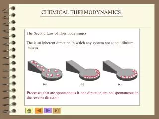
Fig. 4.2: p-T diagram ofthesolvent and the solution(see also Fig. 2.4),DTffreezing point lowering, DTbboiling point elevation
Have a look on Fig. 4.2! There are compared the solvent (black curve) and the solution (red curve) properties in a p-T diagram. The vapor pressure decreasesin comparison of the p-T diagrams of the solvent and the solution. At a constant T’ temperature the p*-p is observable. Theboiling point increases(DTb).On the figure you can see it at atmospheric pressure. In contrary to the behavor of the boiling point thefreezing point decreasesas effect of the solving (DTf).
Dilute solution is ideal for the solvent Molar Gibbs functions Understanding the boiling point elevation based on equivalence of the chemical potentials in equlibrium: (3.24) (4.2)
G = H - TS dG =Vdp -SdT (2.19b) Derivative of a ratio: (4.3) This is the Gibbs-Helmholtz equation, see (3.52).
(molar heat of vaporization) Assume that the molar heat of vaporization is independent of temperature, and integrate from the boiling point of the pure component (Tb) to T.
(4.4) Substitute the mole fraction of the solute:x1 = 1-x2 Take the power series of ln(1-x2), and ignore the higher terms since they are negligible (x2<<1)
(4.5) In dilute liquid solutionsmolality (m= mol solute per kg solvent) orconcentration(molarity) (c= mol solute per dm3 solution) are used (instead of mole fraction).
Includes the parameters of the solvent only: Kb m2: molality of soluteM1: molar mass of solvent With this (4.6) (4.7) Kb:molal boiling point elevation
Examples: Kb(water) = 0.51 K·kg/mol Kb(benzene) = 2.53 K·kg/mol Application: determination of molar mass determination of degree of dissociation These measurements are possible since the boiling point elevation depends on the number of dissolved particles.
4.2.Freezing point depression of dilute solutions The equation of the freezing point curve in dilute solutions has the following form (see equation 3.53): (4.8) x1: mole fraction of solventDHm(fus):molar heat of fusion of solvent T0: freezing point (melting point) of pure solventT: freezing point of solution
Since We have from (4.8) (4.9) LetT0 - T = DT, andT·T0T02 And so we have from (4.9) (4.10) The freezing point depressionis (4.11)
Since x2 m2M1, we have This multipier (Kf)contains solvent parameters only, (4.12) Kfis molal freezing point depression (4.13) The following examples are given in molality units Molality unit: moles solute pro 1 kg solvent Kf(water) = 1.83 K·kg/mol Kf(benzene) = 5.12 K·kg/mol Kf(camphor) = 40 K·kg/mol
4.3. Osmotic pressure Osmosis:two solutions of the same substance with different concentrations are separated by asemi-permeable membrane(a membrane permeable for the solvent but not for the solute). Then the solvent starts to go through the membrane from the more dilute solution towards the more concentrated solution. Why ? Because the chemical potential of the solvent is greater in the more dilute solution. The „more dilute” solution may be a pure solvent, component 1.
If the more concentrated solution cannot expand freely, its pressure increases, increasing the chemical potential. Sooner or lateran equilibrium is attained. (The chemical potential of the solvent is equal in the two solutions.) The measured pressure difference between the two sides of the semipermeable membrane is called osmotic pressure (p). What does osmotic pressure depend on? van´t Hoff found (1885) for dilute solutions (solute:component 2) pV = n2RT (4.14) (4.14) is similar to the ideal gas law, see equ. (1.27) p = c2RT (4.15)
p p m1*(p) (solvent) m1(x1,p+p) membrane The effect of osmotic pressure is illustrated on Fig. 4.3. Fig. 4.3
Interpretation of Fig. 4.3.The condition for equilibrium is (4.16) The right hand side is the sum of a pressure dependent and a mole fraction dependent term: (4.17) The chemical potential of a pure substance (molar Gibbs function) depends on pressure
see (2.19b) For m V1 is thepartial molar volume(see equ. 3.5).Its pressure dependence can be neglected.(The volume of a liquid only slightly changes with pressure), so the integral is only V1p. So we have 0 = pV1 +Dm1(x1) Dm1(x1) = -pV1 (4.18) Rearranged This equation is good both for ideal and for real solutions.Measuring the osmotic pressurewe can determine m (and the activity).
In a dilute solutiona) n2 can be neglected beside n1b) V1 approaches the molar volume of the pure solventc) the contribution of solute to the total volume can be neglected ( ). In an ideal solution:Dm1(x1) = RTlnx1 (3.24) For dilute solution: -lnx1 = -ln(1-x2) x2 pV1 = -RTlnx1 RTx2 (4.19)
With this restrictions the result is the van’t Hoff equationfor the osmotic pressure, in forms (4.20a) (4.20b) The osmotic pressure is an important phenomenon in living organisms. Think on the cell – cell membrane – intercellular solution systems.
4.4 Enthalpy of mixing Mixing is usually accompanied bychange of energy. Mixing processes are studied atconstant pressure. Heat of mixing (Q) = enthalpy of mixing At constant pressure and constant temperature (4.21a) (4.21b) (molar enthalpy of solution)
Molar heat of mixing(called also integral heat of solution, and molar enthalpy of mixing) is the enthalpy change when 1 mol solution is produced from the components at constant temperature and pressure. In case of ideal solutions the enthalpy is additive, Qms= 0, if there is no change of state. In real solutions Qms(molar heat of fusion) is not zero.The next figures present the deviations from the ideal behavior.
Qms 0 1 x2 • Real solution with positive deviation(the attractive forces between unlike molecules are smaller than those between the like molecules). Qms > 0In an isothermal process we must add heat. In an adiabatic process the mixture cooles down. Endothermic process, see section 3.1. Fig. 4.4
Qms 0 1 x2 Real solution with negative deviation(the attractive forces between unlike molecules are greater than those between the like molecules). Qms < 0 In an isothermal process we must distract heat. In an adiabatic process the mixture warmes up. Exothermic process, see section 3.1. Fig. 4.5.
Differential heat of solutionis the heat exchange when one mole of component is added to infinite amount of solution at constant temperature and pressure. Therefore the differential heat of solution is the partial molar heat of solution: (4.22)
Qms 0 1 x2 The determination of the differencial heats of solution is possible e.g. withthe method of intercepts, Fig. 4.6 (see also e.g. Fig. 3.8): x2 Qm1 Fig. 4.6 Qm2
Explanation to Fig. 4.6. [Like (3.2)]: Differentiating with respect to the amount: (4.23) The differencial heat of solution is equal to the partial molar enthalpy minus the enthalpy of pure component. Enthalpy diagrams:the enthalpy of solution is plotted as the function of composition at different temperatures. These diagrams can be used for the calculation of the heat effects of the solutions.
Fig. 4.7 is a model of a solution enthalpy diagram, theethanol - water system. Technical units are used! h (kJ/kg) 80 oC 300 50 oC 0 0 oC wet 0 1 Compare Fig. 4.7 with Fig. 3.2! Fig. 4.7
Fig. 4.8 introduces the isothermal mole fraction depence of heat of solution of the dioxane-water system Fig. 4.8
Isothermal mixing: we are on the same isotherm before and after mixing.(see Fig. 4.8). According to (3.2) we have Qs = (m1+m2)h - (m1h1+m2h2) (4.24) h, h1, h2 can be read from the diagram, using the tangent. Adiabatic mixing: the point corresponding to the solution is on the straight line connecting the two initial states (see Fig. 4.9). Abbreviatons to the figure: the mole fraction of the selected component is denoted by x, A an B are the initial solutions: xA, HmA xB, HmB, nA = n – nB.
Hm B HmB t2 t1 HmA A x 0 xA xB 1 Material balance: (n-nB)xA+nBxB = nx and (n-nB)HmA+nBHmB = nHm Rearranging these equations: nB(xB - xA) = n(x- xA) nB(HmB-HmA) = n(Hm-HmA) Dividing these equations by one another Hm (4.25) (4.25) is a linear equation x Fig. 4.9
At last we have (4.26) This is a straight line crossing the points (x1,y1) and (x2,y2) like the algebraic equation
4.5 Henry’s law In a very dilute solution every dissolved molecule is surrounded by solvent molecules: Fig. 4.10 If a further solute molecule is put into the solution, it will also be surrounded by solvent molecules. It will get into the same molecular environment. So the vapor pressure and other macroscopic properties will be proportional to the mole fraction of the solute: Henry’s law.
p t = const. Raoult p2* Raoult p2 p1* Henry Henry p1 0 x2 1 1 2 Henry’s law is valid for low mole fractions. Fig 4.11, observe deviations! Fig. 4.11
Where component 2 is the solute, the left hand side of Fig. 4.11): (4.27) kH is theHenry constant In the same range the Raoult´s law applies to the solvent: like (3.18) The two equations are similar. There is a difference in the constants. p1* has an exact physical meaning (the vapor pressure of pure substance) while kH does not have any exact meaning. In a dilute solution the Raoult´s law is valid for the solvent and Henry´s law is valid for the solute.
4.6 Solubility of gases The solution of gases in liquids are generally dilute, so we can use Henry´s law. The partial pressure of the gas above the solution is proportional to the mole fraction in the liquid phase. Usually the mole fraction (or other parameter expressing the composition) is plotted against the pressure. If Henry´s law applies, this function is a straight line. See e.g. the solubilty of some gases on Fig. 4.12!
x The solubility of some gases in water at 25 oC 0.01 H2 N2 O2 400 p [bar] Fig. 4.12
In case of N2 and H2 the function is linear up to several hundred bars (Henry´s law applies), in case of O2 the function is not linear even below 100 bar. Absorption - desorption Temperature dependence of solubility of gases Le Chatelier´s principle: a system in equilibrium, when subjected to a perturbation, responds in a way that tends to minimize its effect. Solution of a gas is a change of state: gas liquid. It is usually an exothermic process. Increase of temperature: the equilibrium is shifted towards the endothermic direction desorption. The solubility of gases usually decreases with increasing the temperature.
4.7 Thermodynamic stability of solutions One requirement for the stability is the negative Gibbs function of mixing. The negative Gibbs function of mixing does not necessary mean solubility (see Fig. 4.13d diagram of the next figure). Other requirement:The second derivative of the Gibbs free energy of mixing with respect to composition must be positive.
DmGm DmGm DmGm DmGm 0 0 0 0 x2 x2 x2 x2 Some examples of the dependence of molar Gibbs free energy as a function of mole fraction Complete miscibility Complete immiscibility Limited miscibility Limited miscibility Fig. 4.13d Fig. 4.13a Fig. 4.13b Fig. 4.13c
2. 1. The conditions for stability: (4.28) (4.29) Limited miscibility (diagram 4.13d). Chemical potential: partial molar Gibbs function.Remember!Partial molar quantity of Gibbs function of mixing is the change of chemical potential when mixing takes place: 1 , 2.The chemical potential of a component must be the same in the two phases.
Limited miscibility. At the marked points the first derivative changes it sign from negative to positive, according to the requirements of (4.29). Phase rich in 2 Phase rich in 1 DmGm Dm1 Dm2 0 1 x2 Fig. 4.14
Dm1must be the same in the phase rich in 1 as in the phase rich in 2 according to ther requirement of equilibrium. The same applies toDm2. The common tangent of the two curves producesDm1 and Dm2(method of intercepts). Fig. 4.14.
t [oC] 1 phase 20 tuc 2phases 0 n-hexane nitrobenzene 4.8. Liquid - liquid phase equilibria The mutual solubility depends on temperature. In most cases the solubility increases with increasing temperature. tuc : upper critical solution temperature u: upper In this case the formed complex decomposes at higher temperatures. Fig. 4.15
t [ C] o 60 2 phases 20 tlc 1 phase water triethyl-amine Sometimes the mutual solubility increases with decreasing temperature. tlc : lower critical solution temperature l: lower Solubility is better at low temperature because they form a weak complex, which decomposes at higher temperatures. Fig. 4.16
t [ C] o 1 phase tuc 200 2 phases 60 tlc 1 phase water nicotine In a special case there are both upper and lower critical solution temperatures. Low t: weak complexes Higher t: they decompose At even higher temperatures the thermal motion homogenizes the system. Fig, 4.17 x
4.9 Distribution equilibria We discuss the case when a solute is distributed between two solvents, which are immiscible. In equilibrium the chemical potential of the solute is equal in the two solvents (A and B). (4.30) The chemical potential can be expressed as See (3.25)