Fitting and Registration in Computer Vision: Methods and Challenges
This lecture explores key concepts in fitting and alignment within computer vision, emphasizing techniques like Hough transform for edge detection and circle finding. It covers the development of a texture dictionary for image matching and the implementation of the Expectation-Maximization (EM) algorithm for color distribution estimation and object segmentation. Critical considerations such as outlier sensitivity, noise robustness, and optimization challenges are discussed. Practical examples include least squares fitting and global optimization strategies in image analysis.


Fitting and Registration in Computer Vision: Methods and Challenges
E N D
Presentation Transcript
02/15/11 Fitting and Registration Computer Vision CS 543 / ECE 549 University of Illinois Derek Hoiem
Announcements • HW 1 due today • HW 2 out on Thursday • Compute edges and find circles in image using Hough transform • Create dictionary of texture responses and use it to match texture images • Derive the EM algorithm for a mixture of multinomials • Estimate foreground and background color distributions using EM and segment the object using graph cuts
Fitting: find the parameters of a model that best fit the data Alignment: find the parameters of the transformation that best align matched points
Example: Computing vanishing points Slide from Silvio Savarese
Example: Estimating an homographic transformation H Slide from Silvio Savarese
Example: Estimating “fundamental matrix” that corresponds two views Slide from Silvio Savarese
Example: fitting an 2D shape template A Slide from Silvio Savarese
Example: fitting a 3D object model Slide from Silvio Savarese
Critical issues: noisy data Slide from Silvio Savarese
Critical issues: intra-class variability “All models are wrong, but some are useful.” Box and Draper 1979 A Slide from Silvio Savarese
Critical issues: outliers H Slide from Silvio Savarese
Critical issues: missing data (occlusions) Slide from Silvio Savarese
Fitting and Alignment • Design challenges • Design a suitable goodness of fit measure • Similarity should reflect application goals • Encode robustness to outliers and noise • Design an optimization method • Avoid local optima • Find best parameters quickly
Fitting and Alignment: Methods • Global optimization / Search for parameters • Least squares fit • Robust least squares • Iterative closest point (ICP) • Hypothesize and test • Generalized Hough transform • RANSAC
Least squares line fitting • Data: (x1, y1), …, (xn, yn) • Line equation: yi = mxi + b • Find (m, b) to minimize y=mx+b (xi, yi) Matlab: p = A \ y; Modified from S. Lazebnik
Problem with “vertical” least squares • Not rotation-invariant • Fails completely for vertical lines Slide from S. Lazebnik
Slide modified from S. Lazebnik Total least squares If (a2+b2=1) then Distance between point (xi, yi) is |axi + byi + c| ax+by+c=0 Unit normal: N=(a, b) (xi, yi) proof: http://mathworld.wolfram.com/Point-LineDistance2-Dimensional.html
Slide modified from S. Lazebnik Total least squares If (a2+b2=1) then Distance between point (xi, yi) is |axi + byi + c| Find (a, b, c) to minimize the sum of squared perpendicular distances ax+by+c=0 Unit normal: N=(a, b) (xi, yi)
Slide modified from S. Lazebnik Total least squares Find (a, b, c) to minimize the sum of squared perpendicular distances ax+by+c=0 Unit normal: N=(a, b) (xi, yi) Solution is eigenvector corresponding to smallest eigenvalue of ATA See details on Raleigh Quotient: http://en.wikipedia.org/wiki/Rayleigh_quotient
Recap: Two Common Optimization Problems Problem statement Solution Problem statement Solution (matlab)
Search / Least squares conclusions Good • Clearly specified objective • Optimization is easy (for least squares) Bad • Not appropriate for non-convex objectives • May get stuck in local minima • Sensitive to outliers • Bad matches, extra points • Doesn’t allow you to get multiple good fits • Detecting multiple objects, lines, etc.
Robust least squares (to deal with outliers) General approach: minimize ui(xi, θ) – residual of ith point w.r.t. model parameters θρ – robust function with scale parameter σ • The robust function ρ • Favors a configuration • with small residuals • Constant penalty for large residuals Slide from S. Savarese
Robust Estimator (M-estimator) • Initialize σ=0 • Choose params to minimize: • E.g., numerical optimization • Compute new σ: • Repeat (2) and (3) until convergence
Hypothesize and test • Propose parameters • Try all possible • Each point votes for all consistent parameters • Repeatedly sample enough points to solve for parameters • Score the given parameters • Number of consistent points, possibly weighted by distance • Choose from among the set of parameters • Global or local maximum of scores • Possibly refine parameters using inliers
Hough transform P.V.C. Hough, Machine Analysis of Bubble Chamber Pictures, Proc. Int. Conf. High Energy Accelerators and Instrumentation, 1959 Given a set of points, find the curve or line that explains the data points best y m b x Hough space y = m x + b Slide from S. Savarese
y m 3 5 3 3 2 2 3 7 11 10 4 3 2 3 1 4 5 2 2 1 0 1 3 3 x b Hough transform y m b x Slide from S. Savarese
Hough transform P.V.C. Hough, Machine Analysis of Bubble Chamber Pictures, Proc. Int. Conf. High Energy Accelerators and Instrumentation, 1959 Issue : parameter space [m,b] is unbounded… Use a polar representation for the parameter space y x Hough space Slide from S. Savarese
Hough transform - experiments votes features Slide from S. Savarese
Hough transform - experiments Noisy data Issue: Grid size needs to be adjusted… features votes Slide from S. Savarese
Hough transform - experiments Issue: spurious peaks due to uniform noise features votes Slide from S. Savarese
Hough transform • Fitting a circle (x, y, r)
Hough transform conclusions Good • Robust to outliers: each point votes separately • Fairly efficient (much faster than trying all sets of parameters) • Provides multiple good fits Bad • Some sensitivity to noise • Bin size trades off between noise tolerance, precision, and speed/memory • Can be hard to find sweet spot • Not suitable for more than a few parameters • grid size grows exponentially Common applications • Line fitting (also circles, ellipses, etc.) • Object instance recognition (parameters are affine transform) • Object category recognition (parameters are position/scale)
RANSAC (RANdom SAmple Consensus) : Fischler & Bolles in ‘81. • Algorithm: • Sample (randomly) the number of points required to fit the model • Solve for model parameters using samples • Score by the fraction of inliers within a preset threshold of the model • Repeat 1-3 until the best model is found with high confidence
RANSAC Line fitting example • Algorithm: • Sample (randomly) the number of points required to fit the model (#=2) • Solve for model parameters using samples • Score by the fraction of inliers within a preset threshold of the model • Repeat 1-3 until the best model is found with high confidence Illustration by Savarese
RANSAC Line fitting example • Algorithm: • Sample (randomly) the number of points required to fit the model (#=2) • Solve for model parameters using samples • Score by the fraction of inliers within a preset threshold of the model • Repeat 1-3 until the best model is found with high confidence
RANSAC Line fitting example • Algorithm: • Sample (randomly) the number of points required to fit the model (#=2) • Solve for model parameters using samples • Score by the fraction of inliers within a preset threshold of the model • Repeat 1-3 until the best model is found with high confidence
RANSAC • Algorithm: • Sample (randomly) the number of points required to fit the model (#=2) • Solve for model parameters using samples • Score by the fraction of inliers within a preset threshold of the model • Repeat 1-3 until the best model is found with high confidence
How to choose parameters? • Number of samples N • Choose N so that, with probability p, at least one random sample is free from outliers (e.g. p=0.99) (outlier ratio: e ) • Number of sampled points s • Minimum number needed to fit the model • Distance threshold • Choose so that a good point with noise is likely (e.g., prob=0.95) within threshold • Zero-mean Gaussian noise with std. dev. σ: t2=3.84σ2 modified from M. Pollefeys
RANSAC conclusions Good • Robust to outliers • Applicable for larger number of parameters than Hough transform • Parameters are easier to choose than Hough transform Bad • Computational time grows quickly with fraction of outliers and number of parameters • Not good for getting multiple fits Common applications • Computing a homography (e.g., image stitching) • Estimating fundamental matrix (relating two views)
What if you want to align but have no prior matched pairs? • Hough transform and RANSAC not applicable • Important applications Medical imaging: match brain scans or contours Robotics: match point clouds
Iterative Closest Points (ICP) Algorithm Goal: estimate transform between two dense sets of points • Assign each point in {Set 1} to its nearest neighbor in {Set 2} • Estimate transformation parameters • e.g., least squares or robust least squares • Transform the points in {Set 1} using estimated parameters • Repeat steps 2-4 until change is very small
Example: solving for translation A1 B1 A2 B2 A3 B3 Given matched points in {A} and {B}, estimate the translation of the object
Example: solving for translation (tx, ty) A1 B1 A2 B2 A3 B3 Least squares solution • Write down objective function • Derived solution • Compute derivative • Compute solution • Computational solution • Write in form Ax=b • Solve using pseudo-inverse or eigenvalue decomposition
Example: solving for translation A5 B4 (tx, ty) A1 B1 A4 B5 A2 B2 A3 B3 Problem: outliers RANSAC solution Sample a set of matching points (1 pair) Solve for transformation parameters Score parameters with number of inliers Repeat steps 1-3 N times
Example: solving for translation (tx, ty) A4 B4 B1 A1 A2 B2 B5 A5 A3 B3 B6 A6 Problem: outliers, multiple objects, and/or many-to-one matches Hough transform solution Initialize a grid of parameter values Each matched pair casts a vote for consistent values Find the parameters with the most votes Solve using least squares with inliers
Example: solving for translation (tx, ty) Problem: no initial guesses for correspondence ICP solution Find nearest neighbors for each point Compute transform using matches Move points using transform Repeat steps 1-3 until convergence
Next class: Clustering • Clustering algorithms • K-means • K-medoids • Hierarchical clustering • Model selection