Pipe Networks
Fall 2011. CWR 4540 C. Pipe Networks. Sept 8, 2011. Dr. Kristoph-Dietrich Kinzli Department of Environmental and Civil Engineering Florida Gulf Coast University. Magdeburg Water Bridge. Wasserstraßenkreuz opened in October 2003


Pipe Networks
E N D
Presentation Transcript
Fall 2011 CWR 4540 C Pipe Networks Sept 8, 2011 Dr. Kristoph-Dietrich Kinzli Department of Environmental and Civil Engineering Florida Gulf Coast University
Magdeburg Water Bridge • Wasserstraßenkreuz • opened in October 2003 • connects the Elbe-Havel Kanal to the Mittellandkanal, crossing over the Elbe River. • longest navigable aqueduct in the world, with a total length of 918 meters (3,012 ft) • previously 12-kilometre (7.5 mi) detour, offloading due to water levels in Elbe • 1350 tons vs 800 tons • 500 million Euros – 6 years • 24,000 tons of steel and 68,000 cubic meters of concrete
Introduction – Pipe Networks • The purpose of a water distribution network is to supply the system’s users with the amount of water demanded and to supply this water with adequate pressure under various loading conditions. • Water distribution system have three major components; pumping station, distribution storage and distribution piping. • Performance criteria are generally minimum flow rates and pressure (why?)
Today’s Learning Objectives • Apply continuity and energy equations to pipe system networks • Analyze pipe flow and pressure in a network • Illustrate the iterative solution of the loop equations using the Hardy Cross Method • Develop a spreadsheet to solve a simple water distribution system using the Hardy-Cross method
Nodal Method: Friction loss local losses • The energy equation is written for each pipeline in the network as h1: head at the upstream end of a pipe (m) h2: head at the downstream end of a pipe (m) hp : head added by pumps in the pipeline (m) A : cross-sectional area of a pipe (m2) • Positive flow direction is from node 1 to node 2 • Application is limited to relatively simple networks
Example 2.9 (Chin, pg 41-43) The high-pressure ductile-iron pipeline shown in Figure 2.10 becomes divided at point B and rejoins at point C. The pipeline characteristics are given in the following tables. If the flowrate in Pipe 1 is 2 m3/s and the pressure at point A is 900 kPa, calculate the pressure at point D. Assume that the flows are fully turbulent in all pipes. ks Flowrate(Q) Pressure(P)
Example 2.9 (Chin, pg 41-43) – cont. Step 1: Calculate ks/D and f for each pipe Step 2: Calculate the total energy head at location A, hA Step 3: Write down the energy equations for each pipe Step 4: Use continuity equations at two pipe junctions (Qin = Qout1 + Qout2) Step 5: Determine Q of each pipe and hD Step 6: Determine PD using the calculated hD
In-class activity (Example problem) The pipe system shown in the figure below connects reservoirs that have an elevation difference of 20 m. This pipe system consists of 200 m of 50-cm concrete pipe (pipe A), that branches into 400 m of 20-cm pipe (pipe B) and 400 m of 40-cm pipe (pipe C) in parallel. Pipes B and C join into a single 50-cm pipe that is 500 m long (pipe D). For f = 0.030 in all the pipes, what is the flow rate in each pipe of the system?
Hardy Cross Method (Cross, 1936) • The Hardy Cross method is a simple technique for hand solution of the loop system of equations in pipe networks • The flowrate in each pipe is adjusted iteratively until all equations are satisfied. • The method is based on two primary physical laws: • The sum of pipe flows into and out of a node equals the flow entering or leaving the system through the node. • the algebraic sum of the head losses within each loop is equal to zero. hL,j: head loss in pipe j of a loop hp,j: head added by any pumps in pipe j n : the number of pipes in a loop
For analysis, basic criteria should be followed: • The total flow entering each point (node) must equal to the total flow leaving that joint (node). ΣQin = ΣQout • The flow in a pipe must follow the pipe’s friction law for the pipe. hf = kQn n is coefficient depend on equation used • The algebra sum of the head loss in the pipe network must be zero. Σ hf = 0
For analysis, basic criteria should be followed: Q : flow rate (m3/s), D : pipe diameter (m) L : length of pipe (m) f : friction factor CH : H-W coefficient • General equation for losses, hf = rQn(SI units) • Darcy-Weisbach • Hazen Williams
For analysis, basic criteria should be followed: Q : flow rate (ft3/s), D : pipe diameter (ft) L : length of pipe (ft) f : friction factor CH : H-W coefficient • General equation for losses, hf = rQn(US units) • Darcy-Weisbach • Hazen William
Hardy-Cross Method (Derivation) For Closed Loop: Qa: assumed flowrate ΔQ : error in the assumption Q : actual flowrate If ΔQ is small, higher order terms in ΔQ can be neglected • n=2.0, Darcy-Weisbach • n=1.85, Hazen-Williams
Steps for Q distribution using Hardy Cross method: Step 1: Build up system configuration and assume a reasonable distribution of flows the pipe network. but Q=0 at each node. Step 2: Calculate head loss of each pipe section with D-W or H-W equ. Step 3: Calculate (rQ|Q|n-1) and (n r |Q|n-1) in each loop of the pipe network. Step 4: Get ∆Q value for correction Step 5: Calculate the new flow rate Qnew= Q + ∆Q Step 6: Repeat this step (3 ~ 5) until ∆Q = 0 Step 7: Check the mass and energy balance. Step 8: Compute the pressure distribution in the network and check on the pressure requirement.
Example 2.10 (Chin, pg 46-48) Compute the distribution of flows in the pipe network shown in Figure 2.11 (a), where the head loss in each pipe is given by , and the relative values of r are shown in Figure 2.11 (a). The flows are taken as dimensionless for the sake of illustration. Given condition Assumed Q and direction
In-class activity (Pipe networks)- cont. 25 cfs 100 cfs r = 1 r = 4 Loop I Loop II r = 4 r = 2 r = 3 r = 5 25 cfs 50cfs
In-class activity (Pipe networks)- cont. 25 cfs 61.7 cfs 100 cfs 61.7 cfs r = 1 r = 4 Loop I Loop II r = 4 r = 2 12.1 cfs 14.8 cfs r = 3 38.3 cfs r = 5 25 cfs 35.2 cfs 50cfs
In-class activity (Pipe networks) 1.5 cfs r = 8 r = 15 r = 11 r = 8 0.5 cfs r = 6 r = 25 Determine the flow rate in each pipe of the system with direction, with the data shown! 1 cfs