Download
1 / 46
460 likes | 493 Views
BIOINFORMATICS Sequence to Structure. Mark Gerstein, Yale University gersteinlab.org/courses/452 (last edit in spring '10, edit before class #4). class #3 continues from last ppt. Secondary Structure Prediction Overview. Why interesting?

E N D
BIOINFORMATICSSequence to Structure Mark Gerstein, Yale University gersteinlab.org/courses/452 (last edit in spring '10, edit before class #4)
Secondary Structure Prediction Overview • Why interesting? • Not tremendous success, but many methods brought to bear. • What does difficulty tell about protein structure? • Start with TM Prediction (Simpler) • Basic GOR Sec. Struc. Prediction • Better GOR • GOR III, IV, semi-parametric improvements, DSC • Other Methods • NN, nearest nbr.
What secondary structure prediction tries to accomplish? • Not Same as Tertiary Structure Prediction -- no coordinates • Need torsion angles of terms + slight diff. in torsions of sec. str. Credits: Rost et al. 1993; Fasman & Gilbert, 1990 Sequence RPDFCLEPPYTGPCKARIIRYFYNAKAGLVQTFVYGGCRAKRNNFKSAEDAMRTCGGA Structure CCGGGGCCCCCCCCCCCEEEEEEETTTTEEEEEEECCCCCTTTTBTTHHHHHHHHHCC
TM Helix Identification The problem
Some TM scales: GES KD I 4.5 V 4.2 L 3.8 F 2.8 C 2.5 M 1.9 A 1.8 G -0.4 T -0.7 W -0.9 S -0.8 Y -1.3 P -1.6 H -3.2 E -3.5 Q -3.5 D -3.5 N -3.5 K -3.9 R -4.5 F -3.7 M -3.4 I -3.1 L -2.8 V -2.6 C -2.0 W -1.9 A -1.6 T -1.2 G -1.0 S -0.6 P +0.2 Y +0.7 H +3.0 Q +4.1 N +4.8 E +8.2 K +8.8 D +9.2 R +12.3 Goldman, Engleman, Steitz KD – Kyte Dolittle For instance, DG from transfer of a Phe amino acid from water to hexane
How to use GES to predict proteins • Transmembrane segments can be identified by using the GES hydrophobicity scale (Engelman et al., 1986). The values from the scale for amino acids in a window of size 20 (the typical size of a transmembrane helix) were averaged and then compared against a cutoff of -1 kcal/mole. A value under this cutoff was taken to indicate the existence of a transmembrane helix. • H-19(i) = [ H(i-9)+H(i-8)+...+H(i) + H(i+1) + H(i+2) + . . . + H(i+9) ] / 19 Core
Graph showing Peaks in scales Illustrations Adapted From: von Heijne, 1992; Smith notes, 1997 Core
Ex. P(i,a) probability that residue i has secondary structure a • Problem of DB Bias • f(A) = frequency of residue A to have a TM-helical conf. in db • f(A,i) = f(A) at position i in a particular sequence • E(a)=statistical energy of helix over a window • p(i, a) = probability that residue i is in a TM-helix Core -10 1 20 30 Fin-DB(A) = 5/120 Fin-TM(A) = 3/60 A A A A A
Statistics Based Methods:Persson & Argos • Propensity P(A) for amino acid A to be in the middle of a TM helix or near the edge of a TM helix Core Illustration Credits: Persson & Argos, 1994 P(A) = fTM(A)/fSwissProt(A)
Scale Detail Extra
Add-ons ("hacks"):Removing Signal sequences • Initial hydrophobic stretches corresponding to signal sequences for membrane insertion were excluded. (These have the pattern of a charged residue within the first 7, followed by a stretch of 14 with an average hydrophobicity under the cutoff). Extra
Add-ons: Charge on the Outside, Positive Inside Rule • for marginal helices, decide on basis of R+K inside (cytoplasmic) Ext Cyt Extra Credits: von Heijne, 1992
GOR: Simplifications Core • For independent events just add up the information • I(Sj ; R1, R2, R3,...Rlast) = Information that first through last residue of protein has on the conformation of residue j (Sj) • Could get this just from sequence sim. or if same struc. in DB (homology best way to predict sec. struc.!) • Simplify using a 17 residue window: I(Sj=H ; R[j-8], R[j-7], ...., R[j], .... R[j+8]) • Difference of information for residue to be in helix relative to not: I(dSj;y) = I(Sj=H;y)-I(Sj=~H;y) • odds ratio: I(dSj;y)= ln P(Sj;y)/P(~Sj;y) • I determined by observing counts in the DB, essentially a lod value
Basic GOR • Pain & Robson, 1971; Garnier, Osguthorpe, Robson, 1978 • I ~ sum of I(Sj,R[j+m]) over 17 residue window centered on j and indexed by m • I(Sj,R[j+m]) = information that residue at position m in window has about conformation of protein at position j • 1020 bins=17*20*3 • In Words • Secondary structure prediction can be done using the GOR program (Garnier et al., 1996; Garnier et al., 1978; Gibrat et al., 1987). This is a well-established and commonly used method. It is statistically based so that the prediction for a particular residue (say Ala) to be in a given state (i.e. helix) is directly based on the frequency that this residue (and taking into account neighbors at +/- 1, +/- 2, and so forth) occurs in this state in a database of solved structures. Specifically, for version II of the GOR program (Garnier et al., 1978), the prediction for residue i is based on a window from i-8 to i+8 around i, and within this window, the 17 individual residue frequencies (singlets). -8 0 3 +8 f(H,+3)/f(~H,+3)
The Secondary Structure Prediction Problem Core -8 "Grand Formula" GOR Simplification
GORparameters OBS = F (residue "A" to be at window position j [e.g. =i-3] in a helix centered at position i) EXP = F (residue "A" in the DB in general) OBS LOD= ln ------- EXP
Directional Information helix strand coil Credits: King & Sternberg, 1996 Core
Types of Residues • Group I favorable residues and Group II unfavorable one: • A, E, L -> H; V, I, Y, W, C -> E; G, N, D, S -> C • P complex; largest effect on proceeding residue • Some residues favorable at only one terminus (K) Credits: King & Sternberg, 1996 Core
Updated GOR ("IV") • I(Sj; R[j+m], R[j+n]) = the frequencies of all 136 (=16*17/2) possible di-residue pairs (doublets) in the window. • 20*20*3*16*17/2=163200 pairs • Parameter Explosion Problem: 1000 dom. struc. * 100 res./dom. = 100k counts, over how many bins • Dummy counts for low values (Bayes) Core All Singletons in 17 residue window All Pairs
How to calculate an entry in the simple GOR tables and a comparison to updated GOR (I vs IV) Core
Spectrum of calculations Simple - 20 values at position i Simple GOR - ~1000 values within 17res window at i Updated GOR ~ 160K, all pairs within the window (bin = how many times do I have a helix at i with A at position m=5 and V at position n=-4) GOR-2010 - bigger window, triplets GOR - 5000 -- all 15mer words, 20^15
An example of mini-GOR Also, why secondary structure prediction is so hard Core
Assessment • Q3 + other assess, 3x3 • Q3 = total number of residues predicted correctly over total number of residues (PPV) • GOR gets 65% • sum of diagonal over total number of residue -- (14K+5K+21K)/ 64K • Under predict strands & to a lesser degree, helices: 5.9 v 4.1, 10.9 v 10.6 Credits: Garnier et al., 1996 AASDTLVVIPWERE Input Seq HHHHHEEEECCCHH Pred. hhhheeeeeeeech Gold Std.
Training Set (determine parms)Testing Set (see how it does) Validation SetPredictions from actual run Over-training 4-fold • Cross Validation: Leave one out, seven-fold Credits: Munson, 1995; Garnier et al., 1996
Is 100% Accuracy Possible? Extra Quoted from Barton (1995): The problem of evaluation is more complicated for prediction from multiple sequences, as the prediction is a consensus for the family and so is not expected to be 100% in agreement with any single family member. Simple residue by residue percentage accuracy has long been the standard method of assessment of secondary structure predictions. Although a useful guide, high percentage accuracies can be obtained for predictions of structures that are unlike proteins. For example, predicting myoglobin to be entirely helical (no strand or coil) will give over 80% accuracy but the prediction is of little practical use.
More Types of Secondary Structure Prediction Methods • Parametric Statistical • struc. = explicit numerical func. of the data (GOR) • Non-parametric • struc. = NON- explicit numerical func. of the data • generalize Neural Net, seq patterns, nearest nbr, &c. • Semi-parametric: combine both • single sequence • multi sequence • with or without multiple-alignment Core
GOR Semi-parametric Improvements • Filtering GOR to regularize Core Illustration Credits: King & Sternberg, 1996
Multiple Sequence Methods • Average GOR over multiple seq. Alignment • The GOR method only uses single sequence information and because of this achieves lower accuracy (65 versus >71 %) than the current "state-of-the-art" methods that incorporate multiple sequence information (e.g. King & Sternberg, 1996; Rost, 1996; Rost & Sander, 1993). Illustration Credits: Livingston & Barton, 1996
DSC -- an improvement on GOR • GOR parms • + simple linear discriminant analysis on: • dist from C-term, N-term • insertions/deletes • overall composition • hydrophobic moments • autocorrelate: helices • conservation moment Illustration Credits: King & Sternberg, 1996
Conservation, k-nn Extra outside Patterns of Conservation Inside (conserved) k-nearest neighbors
Neural Networks • Somehow generalize and learn patterns • Black Box • Perceptron (above) is Simplest network • Multiply junction * input, sum, and threshold Extra Illustration Credits: Rost & Sander, 1993
More NN • Hidden Layer • Learning • Steepest descent to minimize an error function • Jury Decision • Combine methods • Escape initial conditions Extra Illustration Credits: D Frishman handout
Yet more methods…. • struc class predict • Vect dist. between composition vectors • threading via pair pot • Distant seq comparison • ab initio from md • ab initio from pair pot. Extra
Fold recognition Query sequence Library of known folds Best-fit fold
Why fold recognition? • Structure prediction made easier by sampling 1,000~10,000 folds, rather than >4100 possible conformations • Practical importance: fold assignment in genomes • Fold recognition can be done using sequence-based (BLAST, HMM, profile alignment) or structure-based methods (threading)
Fold recognition by threading • Input: A query sequence, a fold library • For each fold template in the library: • Generate alignments between the query sequence and the fold template • Evaluate alignments; choose the best one • Do this for all folds, choose the best fold
What is threading • Query sequence: • Thread the sequence onto the fold template • Use structural properties to evaluate the fit • Environment • Pairwise interactions
Align sequence to fold: an example 1 12 13 2 ● Align: RVLGFIPTWFALSKY to: Many possible alignments: 11 4 3 14 15 6 10 5 9 7 8 16 A L R L S V R A L F S R V L G A K F L L G W S K V I F F Y K Y F G W F T P T W Y P I P I T 123456789012--3456 RVLGF--IPTWFALSKY- 1234567890123456 RVLGFIPTWFALSKY- 1234567890123456 -RVLGFIPTWFALSKY DeletionInsertion
Evaluate alignments using threading energy function • Etotal = Eenv + Epair + Egap • Eenv: Total environment energies. Measures compatibility of a residue and its corresponding 3D environment (secondary structure, solvent accessibility) • Epair: Total pairwise energies. Measures interaction between spatially close residues • Egap: Gap opening and extension penalities
Relationship to Generalized Similarity Matrix • PAM(A,V) = 0.5 • Applies at every position • S(aa @ i, aa @ J) • Specific Matrix for each pair of residues i in protein 1 and J in protein 2 • Example is Y near N-term. matches any C-term. residue (Y at J=2) • S(i,J) • Doesn’t need to depend on a.a. identities at all! • Just need to make up a score for matching residue i in protein 1 with residue J in protein 2 i J
Find the best alignment • NP-hard problem; needs approximation • Dynamic programming and the “frozen approximation” • Approximately calculate amino acid preferences for each residue position by fixing the interaction partners at that position • Find best alignment using dynamic programming • Update interaction partners for each position; repeat till convergence • Other optimization techniques • Simulated annealing • Branch-and-bound, etc.