Download
1 / 54
540 likes | 565 Views
Explore a case study on baboon behavior with a statistical analysis using permutation tests and examine the significance of infant handling. Learn statistical lessons through analyzing female baboon interactions.

E N D
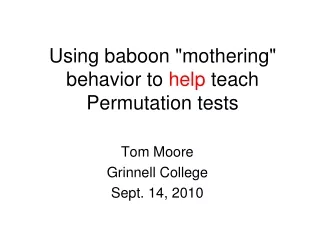
Using baboon "mothering" behavior to help teach Permutation tests Tom Moore Grinnell College Sept. 14, 2010
Plan for presentation • A case study in baboon behavior • Descriptive analysis • The question of statistical significance • Review permutation tests • Finish baboon case study • Statistical lessons
See previous CAUSE webinar: • "Concepts of Statistical Inference: A Randomization-Based Curriculum"with Allan Rossman & Beth Chance, Cal Poly - San Luis Obispo; John Holcomb, Cleveland State University • 2:00 to 2:30 pm Eastern time, April 14th, 2009
The data (handout Table 1) HANDLERS ranks INFANTS/ KM KN NQ PO HQ LL NY PS SK ST WK AL CO DD LS LY MH ML MM PA PH PT RS Mothers 1 1 1 1 | 2 2 2 2 2 2 2 | 3 3 3 3 3 3 3 3 3 3 3 3 ranks KG/KM 1 0 0 4 1 | 1 0 0 0 3 1 0 | 0 0 0 0 0 0 0 0 0 0 2 1 HZ/HQ 2 13 23 7 5 | 0 2 1 1 5 6 18 | 1 6 3 0 1 4 1 0 9 0 10 1 LC/LL 2 4 0 1 4 | 3 0 2 1 1 5 3 | 1 0 0 1 0 2 1 1 1 0 1 6 NK/NY 2 12 4 10 5 | 9 1 0 2 3 11 7 | 8 6 3 1 0 2 1 1 5 3 2 3 PZ/PS 2 1 3 4 1 | 0 0 0 0 0 0 2 | 0 2 0 0 0 3 0 1 1 0 3 0 CY/CO 3 2 2 7 3 | 1 1 2 0 3 12 16 | 3 0 2 0 0 2 0 0 1 0 0 2 LZ/LS 3 1 0 3 2 | 1 1 0 0 2 0 5 | 2 2 2 0 1 9 2 0 0 0 3 2 MQ/ML 3 0 1 5 2 | 2 4 2 2 2 4 5 | 7 5 2 1 1 7 0 4 4 1 0 2 MW/MH 3 3 0 7 4 | 2 3 0 5 2 8 13 | 7 14 2 0 0 0 4 0 8 0 13 6 MX/MM 3 2 3 4 5 | 0 0 0 0 0 5 2 | 9 3 1 0 0 2 0 0 1 2 2 3 PK/PH 3 2 0 6 4 | 3 4 1 0 0 15 10 | 8 5 1 0 3 1 1 6 3 0 7 5
High-ranked female handles mid-ranked infant: Female NQ handles Infant NK 10 timesNK’s mother is NY HANDLERS ranks KM KN NQ PO HQ LL NY PS SK ST WK AL CO DD LS LY MH ML MM PA PH PT RS 1 1 1 1 | 2 2 2 2 2 2 2 | 3 3 3 3 3 3 3 3 3 3 3 3 INFANTS/ Mothers ranks KG/KM 1 0 0 4 1 | 1 0 0 0 3 1 0 | 0 0 0 0 0 0 0 0 0 0 2 1 HZ/HQ 2 13 23 7 5 | 0 2 1 1 5 6 18 | 1 6 3 0 1 4 1 0 9 0 10 1 LC/LL 2 4 0 1 4 | 3 0 2 1 1 5 3 | 1 0 0 1 0 2 1 1 1 0 1 6 NK/NY 2 12 4 10 5 | 9 1 0 2 3 11 7 | 8 6 3 1 0 2 1 1 5 3 2 3 PZ/PS 2 1 3 4 1 | 0 0 0 0 0 0 2 | 0 2 0 0 0 3 0 1 1 0 3 0 CY/CO 3 2 2 7 3 | 1 1 2 0 3 12 16 | 3 0 2 0 0 2 0 0 1 0 0 2 LZ/LS 3 1 0 3 2 | 1 1 0 0 2 0 5 | 2 2 2 0 1 9 2 0 0 0 3 2 MQ/ML 3 0 1 5 2 | 2 4 2 2 2 4 5 | 7 5 2 1 1 7 0 4 4 1 0 2 MW/MH 3 3 0 7 4 | 2 3 0 5 2 8 13 | 7 14 2 0 0 0 4 0 8 0 13 6 MX/MM 3 2 3 4 5 | 0 0 0 0 0 5 2 | 9 3 1 0 0 2 0 0 1 2 2 3 PK/PH 3 2 0 6 4 | 3 4 1 0 0 15 10 | 8 5 1 0 3 1 1 6 3 0 7 5
Plan for presentation • A case study in baboon behavior • Descriptive analysis • The question of statistical significance • Review permutation tests • Finish baboon case study • Statistical lessons
High-ranked female handles mid-ranked infant: Female NQ handles Infant NK 10 timesNK’s mother is NY KM KN NQ PO HQ 1 1 1 1 | 2 INFANTS/ Mothers ranks KG/KM 1 0 0 4 1 | 1 HZ/HQ 2 13 23 7 5 | 0 LC/LL 2 4 0 1 4 | 3 NK/NY 2 12 4 10 5 | 9 PZ/PS 2 1 3 4 1 | 0
High-ranked female handles mid-ranked infant: Female NQ handles Infant NK 10 timesNK’s mother is NY KM KN NQ PO HQ 1 1 1 1 2 KG/KM 1 0 0 4 1 1 HZ/HQ 2 13 23 7 5 0 LC/LL 2 4 0 1 4 3 NK/NY 2 12 4 10 5 9 PZ/PS 2 1 3 4 1 0
Dominance scores • The data are related to interactions between two females and the infant of one of them, i.e., triads • But dominance scores are determined by a prior set of observations involving just two females, i.e., dyads. • Dominance scores range between -22 and 22, but we create from them a categorical variable of High(1), Mid(2), and Low(3) ranks.
The variables • Handler rank: high(1), mid(2), low(3) • Infant rank: high(1), mid(2), low(3) • The number of interactions between a given infant-handler pair
Primary question Is infant handling behavior related to the dominance hierarchy rankings of females in the troop?
Research hypotheses • Females will tend to handle the infants of females who are ranked the same as or lower than themselves. (RH1) • Females will tend to handle the infants of females who are ranked directly below them (or same rank if female is low-ranked). (RH2)
The data (handout) HANDLERS ranks INFANTS/ KM KN NQ PO HQ LL NY PS SK ST WK AL CO DD LS LY MH ML MM PA PH PT RS Mothers 1 1 1 1 | 2 2 2 2 2 2 2 | 3 3 3 3 3 3 3 3 3 3 3 3 ranks KG/KM 1 0 0 4 1 | 1 0 0 0 3 1 0 | 0 0 0 0 0 0 0 0 0 0 2 1 HZ/HQ 2 13 23 7 5 | 0 2 1 1 5 6 18 | 1 6 3 0 1 4 1 0 9 0 10 1 LC/LL 2 4 0 1 4 | 3 0 2 1 1 5 3 | 1 0 0 1 0 2 1 1 1 0 1 6 NK/NY 2 12 4 10 5 | 9 1 0 2 3 11 7 | 8 6 3 1 0 2 1 1 5 3 2 3 PZ/PS 2 1 3 4 1 | 0 0 0 0 0 0 2 | 0 2 0 0 0 3 0 1 1 0 3 0 CY/CO 3 2 2 7 3 | 1 1 2 0 3 12 16 | 3 0 2 0 0 2 0 0 1 0 0 2 LZ/LS 3 1 0 3 2 | 1 1 0 0 2 0 5 | 2 2 2 0 1 9 2 0 0 0 3 2 MQ/ML 3 0 1 5 2 | 2 4 2 2 2 4 5 | 7 5 2 1 1 7 0 4 4 1 0 2 MW/MH 3 3 0 7 4 | 2 3 0 5 2 8 13 | 7 14 2 0 0 0 4 0 8 0 13 6 MX/MM 3 2 3 4 5 | 0 0 0 0 0 5 2 | 9 3 1 0 0 2 0 0 1 2 2 3 PK/PH 3 2 0 6 4 | 3 4 1 0 0 15 10 | 8 5 1 0 3 1 1 6 3 0 7 5 [,1] [,2] [,3] [1,] 5 5 3 [2,] 97 83 95 [3,] 68 138 184
X=handler rank; Y=Infant rank Handler's rank Hi Mid Low Infant Hi 5 5 3 Rank Mi 97 83 95 Lo 68 138 184 Totals: 170 226 282 (A)Counts Handler's rank Hi Mid Low Infant Hi 2.9% > 2.2% > 1.1% Rank Mi 57.1% > 36.7% > 33.9% Lo 40.0% < 61.1% < 65.0% (B)Column%
Residuals Handler's rank Hi Mid Low Infant Hi 0.96 0.32 -2.33 Rank Mi 3.38 -0.91 -1.81 Lo -3.01 0.70 1.71
Residuals Handler's rank Hi Mid Low Infant Hi 0.96 0.32 -2.33 Rank Mi 3.38 -0.91 -1.81 Lo -3.01 0.70 1.71 Is the result Statistically Significant?
Plan for presentation • A case study in baboon behavior • Descriptive analysis • The question of statistical significance • Review permutation tests • Finish baboon case study • Statistical lessons
Permutation test: simpler example • Do birds react to observer clothing color? • Species-confidence hypothesis • Field experiment (1997): • Treatments: vest worn vs. vest not worn • Response: approach distance • n=19 different transects, widely spaced • Transects are randomly allocated to “vests” or “no vests.”
Summary data • Approach distance is greater when vest is worn. • Is the difference statistically significant?
Assessing statistical significance • Statistical significance means “we cannot attribute the observed difference to random allocation alone.” • H0: “Vest mean distance” = “No-vest mean distance” (Null hypothesis) • Ha: “Vest mean distance” > “No-vest mean distance” (Alternative hypothesis)
The test for statistical significance using a permutation test • Assume chance alone, i.e., assume H0 is true; • Then “vest” and “no vest” are merely labels that the experimenter has randomly assigned to the 19 outcomes; • So simulate this process of random assignment many times and form a distribution of mean differences.
Distance group(1=vest, 0= no vest) 14.20 1 13.69 1 3.12 1 15.40 1 9.67 1 mean = 16.68 19.01 1 20.38 1 26.67 1 21.21 1 observed mean 23.40 1 difference = 6.52 11.94 0 11.27 0 8.81 0 6.09 0 8.18 0 mean = 10.16 13.92 0 6.38 0 13.25 0 11.62 0
Distance Random assign re-arrange mean difference 14.20 0 3.12 1 13.69 0 9.67 1 3.12 1 21.21 1 15.40 0 23.40 1 9.67 1 11.27 1 mean = 11.89 19.01 0 8.81 1 20.38 0 6.09 1 26.67 0 8.18 1 21.21 1 13.92 1 23.40 1 13.25 1 diff = 11.94 0 14.20 0 -3.59 11.27 1 13.69 0 8.81 1 15.40 0 6.09 1 19.01 0 8.18 1 20.38 0 mean = 15.48 13.92 1 26.67 0 6.38 0 11.94 0 13.25 1 6.38 0 11.62 0 11.62 0
p-value and statistical significance • P(mean diff ≥ observed mean diff) = the p-value of the test; • of the 100,000 mean differences in the simulation, 908 were ≥ observed difference of 6.52; • so the p-value is empirically estimated to be .00908;
Drawing a conclusion from a p-value • p-value = .009 says that “random allocation alone” is very unlikely to produce a difference as extreme as we observed in the data; • The results are statistically significant • We need some other way to explain this large a mean difference, such as … • The wearing—or not—of an orange vest.
p-value for t=2.613 and 17 degrees of freedom is 0.0091; • essentially identical to permutation p-value; • Generally the permutation result can be approximated by the t
A fact discovered … • nearly 100 years ago by: • R.A. Fisher and • E.J.G. Pitman; • Fisher’s design of experiments book asserted this fact; • Pitman provided the mathematical derivation; • I give references in the last slide.
Interesting bit of history • Pitman wrote in paper: “The main idea is not new, it seems to be implicit in all Fisher’s writings.” • Pitman later said: “I was always dissatisfied with the sentence I wrote ... I wanted to say I really was doing something new.” • Pitman’s contribution was new and it was too bad he ceded credit for it to Fisher.
Plan for presentation • A case study in baboon behavior • Descriptive analysis • The question of statistical significance • Review permutation tests • Finish baboon case study • Statistical lessons
Warblers vs Baboons examples • Warblers data structure is simpler; • Warblers example is a designed experiment, so that statistical significance implies a causal effect; • Baboons example is an observational (non-experimental) study, so statistical significance can at best suggest the presence of a biological mechanism; • with either example, we use a computer simulation to estimate the p-value, but … • with warblers, a t-distribution provides a simpler method of calculating the p-value.
The Null Hypothesis implies … The female handlers interacted with infants as given in the data set. These interactions involved a variety of complex causes, but none of this complexity had anything to do with ranks. That is, ranks can be viewed as meaningless labels attached to infants and females.
With observational data … “…if the data are consistent with a properly constructed null model we can infer that the biological mechanism is not operating, but if the data are inconsistent with the null model, “...this provides some positive evidence in favor of the mechanism.” (Gotelli and Graves, Null Models in Ecology, 1996)
Computing a permutation test • Choose a test statistic, C, which reflects the version of research hypothesis being tested, RH1 or RH2. • (1) Assign ranks at random to infants and females using the rank distributions of the data set. That is, assign ranks at random so that infants are assigned, in this case, 1 High, 4 Mid, and 6 Low and so that females are assigned 4 High’s, 7 Mid’s, and 12 Low’s. This assignment leads to the original data table but with permuted ranks. • (2) Re-form the 3-by-3 table. • (3) Compute the value of C for this table. • Iterate (1)-(3) many times for empirical null distribution.
A sample permutation (Table 2) HANDLERS ranks KM KN NQ PO HQ LL NY PS SK ST WK AL CO DD LS LY MH ML MM PA PH PT RS 1 3 1 3 3 3 2 2 3 1 3 2 2 3 3 1 3 3 3 2 2 3 2 INFANTS/ Mothers ranks KG/KM 1 0 0 4 1 | 1 0 0 0 3 1 0 | 0 0 0 0 0 0 0 0 0 0 2 1 HZ/HQ 3 13 23 7 5 | 0 2 1 1 5 6 18 | 1 6 3 0 1 4 1 0 9 0 10 1 LC/LL 3 4 0 1 4 | 3 0 2 1 1 5 3 | 1 0 0 1 0 2 1 1 1 0 1 6 NK/NY 2 12 4 10 5 | 9 1 0 2 3 11 7 | 8 6 3 1 0 2 1 1 5 3 2 3 PZ/PS 2 1 3 4 1 | 0 0 0 0 0 0 2 | 0 2 0 0 0 3 0 1 1 0 3 0 CY/CO 2 2 2 7 3 | 1 1 2 0 3 12 16 | 3 0 2 0 0 2 0 0 1 0 0 2 LZ/LS 3 1 0 3 2 | 1 1 0 0 2 0 5 | 2 2 2 0 1 9 2 0 0 0 3 2 MQ/ML 3 0 1 5 2 | 2 4 2 2 2 4 5 | 7 5 2 1 1 7 0 4 4 1 0 2 MW/MH 3 3 0 7 4 | 2 3 0 5 2 8 13 | 7 14 2 0 0 0 4 0 8 0 13 6 MX/MM 3 2 3 4 5 | 0 0 0 0 0 5 2 | 9 3 1 0 0 2 0 0 1 2 2 3 PK/PH 2 2 0 6 4 | 3 4 1 0 0 15 10 | 8 5 1 0 3 1 1 6 3 0 7 5 [,1] [,2] [,3] [1,] 5 1 7 [2,] 85 60 119 [3,] 81 117 203
A sample permutation (handout) HANDLERS ranks KM KN NQ PO HQ LL NY PS SK ST WK AL CO DD LS LY MH ML MM PA PH PT RS 1 3 1 3 3 3 2 2 3 1 3 2 2 3 3 1 3 3 3 2 2 3 2 INFANTS/ Mothers ranks KG/KM 1 0 0 4 1 | 1 0 0 0 3 1 0 | 0 0 0 0 0 0 0 0 0 0 2 1 HZ/HQ 3 13 23 7 5 | 0 2 1 1 5 6 18 | 1 6 3 0 1 4 1 0 9 0 10 1 LC/LL 3 4 0 1 4 | 3 0 2 1 1 5 3 | 1 0 0 1 0 2 1 1 1 0 1 6 NK/NY 2 12 4 10 5 | 9 1 0 2 3 11 7 | 8 6 3 1 0 2 1 1 5 3 2 3 PZ/PS 2 1 3 4 1 | 0 0 0 0 0 0 2 | 0 2 0 0 0 3 0 1 1 0 3 0 CY/CO 2 2 2 7 3 | 1 1 2 0 3 12 16 | 3 0 2 0 0 2 0 0 1 0 0 2 LZ/LS 3 1 0 3 2 | 1 1 0 0 2 0 5 | 2 2 2 0 1 9 2 0 0 0 3 2 MQ/ML 3 0 1 5 2 | 2 4 2 2 2 4 5 | 7 5 2 1 1 7 0 4 4 1 0 2 MW/MH 3 3 0 7 4 | 2 3 0 5 2 8 13 | 7 14 2 0 0 0 4 0 8 0 13 6 MX/MM 3 2 3 4 5 | 0 0 0 0 0 5 2 | 9 3 1 0 0 2 0 0 1 2 2 3 PK/PH 2 2 0 6 4 | 3 4 1 0 0 15 10 | 8 5 1 0 3 1 1 6 3 0 7 5 [,1] [,2] [,3] [1,] 5 1 7 [2,] 85 60 119 [3,] 81 117 203
Conclusion • P-value ≈ 15/1000 = .015 • Observed pattern is unlikely the result of chance alone.
Results for All and Successful LTE LT n All 0.015 0.038 678 Succ 0.372 0.017 112 --------------------------- p-values using two test statistics: LTE = less than or equal to; LT = less than
Interpretation of results • Infant-handling as a way to dominate. • Infant-handling as “status striving” • Data supports a nuanced give-and-take between infant handling as nurturing for infant and infant handling as dangerous to infant.