Download
1 / 145
1.5k likes | 2.14k Views
The Economics of Electric Power Networks. Steven Stoft March 5 − 16, 2007 Master Erasmus Mundus EMIN, Paris. Four problems. 1. Find the best prices for dispatch and consumption 2. Find the best prices for investment (in an ideal world)

E N D
The Economics ofElectric Power Networks Steven Stoft March 5 − 16, 2007 Master Erasmus Mundus EMIN, Paris
Four problems 1. Find the best prices for dispatch and consumption 2. Find the best prices for investment (in an ideal world) 3. Can the market solve the reliability problem? 4. Transmission investment: Is the market better than planning? • These are the 4 main economic problems of electricity markets. • All problems are part engineering and part economics. • System security is a fifth problem—but mostly an engineering problem. • Electricity is the only network with prices that change every 10 minutes. • Can these same prices work for 30 year investments?
Measuring electric power & energy • 1 kW = 1 kilowatt = 1,000 Watts = Power 1 kW will power ten 100-Watt lights. 1 kW will burn out one 100-Watt light in a flash. • 1 kWh = 1 kilowatt-hour = Energy 1 kWh will power ten 100-Watt lights for 1 hour. 1 kWh will power one 100-Watt light for 10 hours. • 1 MW = 1 megawatt = 1,000 kW • 1 GW = 1 gigawatt = 1,000 MW ( 1 mW = 1 / 1000 Watts ) PSE, Ch. 1-3
Types of power plants Gas CC = Combined Cycle = gas turbine + steam turbine. Cost = Fixed costs as a one-time cost. Output / Size = Capacity Factor. FC / Cap = Fixed cost per MWh of capacity FC / Out = Fixed cost per MWh of output Plant cost data are from US DOE. Currency conversion = 1.3 dollar / euro. * Capacity factors can vary widely between plants. PSE, Ch. 1-3
Fixed cost units: € / MWh ? • All calculations will use € / MWh for both fixed and marginal cost. • This is unusual, but simple and correct. • Suppose a 1MW line or generator cost 60,000 €. • To rent it would cost ~ 8760 € / year.* (discount rate, taxes and 20-year payback period) • There are 8760 hours / year. • Rental cost = 1€ per hour for each MW. = 1€ / hour / MW = 1€ / MWh. * A business calculation, not adjusted for inflation or technical progress. PSE, Ch. 1-3.1
Introduction to electricity GW • Electricity flows from the power plant to the consumer at 200,000 km/second, and cannot be stored. • Some power plants must constantly change their output. California ISO Load, Feb. 26 • Coal plants “ramp” up and down slowly, ~3 MW / minute • Gas turbines (GTs) and hydro ramp up and down quickly.
PJM’s load duration curve, 2005 GW For example, PJM’s Load was greater than 90 GW 20% of the time during 2005. PSE, Ch. 1-4
Generating Stations (power plants) and Transmission Lines (the grid) Pink lines are 400kV (??) Sparks jump 1 cm in dry air for each 10 kV.
AC power: the ultimate network • Electric power flows through the space around the power lines in an electromagnetic field. • This field rotates 60 times per second like the rotating steel shaft which carries power from your car’s engine to it’s wheels—but it is much stronger. • All generators are connected to this rotating field and rotate exactly together even when 1000’s of km apart. • A connected generator cannot be stopped without breaking it. (To stop, first disconnect.) • The AC network is one giant machine connecting every power plant to every home.
Typical electricity market P Demand Supply Old GTs Market clearing price System MC GT “scarcity rent” “inframarginal rent” Covers FC CC coal nuclear Q
Some basic economics for electricity Assume competitive supply and competitive demand curves. P P Supply Supply Demand Demand 18 € 10 € 9 € Q Q Competitive price = 9 €. MC = 9 € MV = 9 € Competitive price = 18 €. Marginal value = 18 €. The marginal cost is ambiguous, but: 10 € < MC < infinity. Many say that competitive price > MC. This is false. PSE, Ch. 1-6
Reality is simpler It’s simple to think the supply curve is absolutely vertical, but this makes the math more difficult because MC goes to infinity with an infinitesimal change of output. In reality, MC goes from low (~30 €) to infinity with about a 3% change in output. There is no discontinuity. The math is simple and ordinary. High MC = probability of breakdown × the cost of a breakdown. P Supply Demand Not vertical 18 € 10 € Q Competitive price = 18 €. Marginal value = 18 €. Marginal cost = 18 €. No ambiguity! PSE, Ch. 1-6
A dangerous confusion • If there is no market power, P = MC. • If P = MC, peakers cannot cover FC. • This proves “We need market power.” • Some market power is good. • When the price is high, it is impossible to tell if it is from good market power or bad market power. • To find bad market power, you must watch profits for years. • It’s bad to watch profits—they are private. • Looking for market power is a bad idea.
The truth about market power • In a well-designed market • No market power is needed (none, zero). • Market power is bad. • The perfectly competitive price can cover all FC. • Every market has some market power. • A little market power does little harm. • Don’t worry about a little, but don’t encourage it. • Monitor the market for significant market power. ( Lecture 3 will cover the problem of “no competitive price,” but market power is still not needed.)
Problem #1 Prices for Dispatch and Consumption Contents
The old central dispatch problem • Some generators cost more to run. • Some are in the wrong location. • Minimize the cost of the dispatch. • The Old Solution: • Collect all the cost and transmission-line data. • Solve a linear program. • Tell each power plant when to start and how much to produce. PSE, Ch. 3-5,6,7
New central dispatch problem • Find the prices that will cause • power plants to produce power a least cost • and consumers to use power efficiently. • The New Solution: • Have power plants bid: • Marginal cost, Startup cost, … ? • Collect transmission data. • Solve for the competitive prices. PSE, Ch. 3-5,6,7
The role of central dispatch • Without central control: • consumers could steal electricity. • the traders would melt the transmission lines. • The system operator (SO) controls the system • With a market, does the SO need to set prices? • No. Pravin Varaiya (UC Berkeley) has shown that the SO could just limit bilateral trades to protect the power lines and the market could figure out the prices. • This has never been tried. • Pure bilateral trading would probably be less efficient. • That’s why we have stock exchanges. PSE, Ch. 3-5,6,7
Competitive locational prices, CLPs • Prices used for dispatch are called • “nodal prices,” “locational prices” • Nodal prices may not be competitive prices. CLPsare efficient. True. Nodal prices are efficient. May be false. • CLP is my term. If I am talking about competitive prices, I will say CLPs, otherwise, I may say, “nodal.” PSE, Ch. 3-1.3
Are CLPs “centralized prices”? • No. • The are just ordinary competitive prices. • They can come from a centralized auction. • They can come from bilateral trading. ( Bilateral trading is trading between two parties rather than trading with an exchange or a central market. )
What are CLPs like? • They depend on the physics of power flow and transmission limits. • They seem wrong to most people, and most people don’t like them. • When they are not all the same, a big market may have 2000 different prices. • They change every 5 or 10 minutes. • The are the only prices that cause efficient dispatch, investment, and consumption.
Finding CLPs: an example • Two regions with many small generators • Many small connecting lines. Different owners • What are the competitive prices for • Power in the remote location? • Power in the city? • Use of a power line? 500 1-MW power lines MC = marginal cost Mostly fuel, some variable maintenance All cost are in $ / MWh, unless noted. MC = 20 + Q/50 Load = 100 MC = 40 + Q/50 Load = 800 A: Country B: City PSE, Ch. 5-3.1
Finding CLPs: an example • Power will be more expensive in the city, so city folks will pay to use a line and buy power from the country. They will pay PB – PA, but no more. • PT = PB – PA • Does PT = 0, or is PT > 0 ?? 500 1-MW power lines PT > 0 means the lines are congested. (More transmission would be used if available.) MC = 20 + Q/50 Load = 100 Price = PA MC = 40 + Q/50 Load = 800 Price = PB Price = PT Country City PSE, Ch. 5-3.1
Finding CLPs: an example • Assume there is no congestion • If all 900 MW is bought at “A”, the competitive price would be 20 + 900/50 = 38 € / MWh. • If possible, everyone will buy power from A. • They would need 800 MW of transmission to the city. 500 1-MW power lines MC = 20 + Q/50 Load = 100 Price = PA MC = 40 + Q/50 Load = 800 Price = PB Transmission is scarce. PT > 0. The lines are congested. Price = PT Country City PSE, Ch. 5-3.1
Finding CLPs: an example • The city will buy 500 MW from the country and 300 MW in the City. • PB = 40 + 300/50 = 46 € / MWh • Country generators will sell 500 + 100 MW. • PA = 20 + 600/50 = 32 € / MWh • PT = 14 € / MWh 500 1-MW power lines MC = 20 + Q/50 Load = 100 Price = PA MC = 40 + Q/50 Load = 800 Price = PB PT = 46 € – 32€ = 14€/MWh PT > 0 The lines are congested. Price = PT Country City PSE, Ch. 5-3.1
CLPs are bilateral prices • There was no central market in our example. • Only bilateral traders. • CLPs are simply competitive market prices. • They can also be computed from competitive bids in a central market. PSE, Ch. 5-3.1
Properties of the CLPs • CLPs give • The cheapest dispatch (given consumption). • The most valuable consumption (given the dispatch). • CLP = marginal cost of generators at the location of the price. • CLPs are just normal competitive market prices. • If sellers have market power, the locational (nodal) prices will not be CLPs. PSE, Ch. 5-3.2
Networks with loops The dots are “nodes” or “buses.” Networks with Loops Radial Networks (no loops) difficult simple A meshed network (lots of loops) PSE, Ch. 5-4.1
Water or DC current = Light, or Water Turbine 1 Ohm of Resistance + 5 Volts, or + 5 kg/cm2 5 Amps 5 Amps 10 Amps + 10 Volts, or + 10 kg/cm2 0 Volts, or 0 kg/cm2 + − 10 V Battery, or Water Pump 15 Amps 15 liters/second PSE, Ch. 5-1.1
Kirchhoff’s laws & Ohm’s law 1. The net current flow into a node = 0. Example: lower left: 15 – 5 – 10 = 0 2. The net voltage drop around a loop = 0. around the triangle: (10–5) + (5–0) + (0–10) = 0 • Ohm’s Law: V = I·R voltage drop = current × resistance • These are the laws of current flow in a network • They are the same for electrons and water. Benjamin Franklin was wrong. Electrons are negative, so they flow in the opposite direction to his electrical “current.” PSE, Ch. 5-1.1
Electrical power flow Power flows much like water. Power lines have “impedance,” which is like “resistance.” Unlike water or electrical current, there are power “losses.” Some of the power heats the wires. Usually we ignore losses. 5 MW 5 MW 10 MW 15 MW (a bit less) 15 MW Generator Consumer “Load” PSE, Ch. 5-4
Electrical power flow Consumer “Load” For two paths from point A to B, if one has twice the impedance, it will have half the power flow. Each of the three power lines in this diagram has the same impedance. 12 MW 8 MW 4 MW 4 MW 12 MW Generator PSE, Ch. 5-4
The “ principle of superposition” Consumer “Load” Two possible power flows can be added to find a new possible power flow. This is called the DC approximation. It is almost perfect for small power flows on AC lines. 12 MW 13 MW 1 MW 14 MW 15 MW (a bit less) 27 MW Generator Consumer “Load” PSE, Ch. 5-4
An impossible flow Consumer “Load” If the lines have equal impedance this flow is impossible. Without very expensive “phase shifters,” engineers cannot control where the power flows except by turning generators on and off. 12 MW 10 MW 2 MW 17 MW 15 MW (a bit less) 27 MW Generator Consumer “Load” PSE, Ch. 5-4
Simplest looped CLP problem CLP = 30 100 MW load Problem: Find the 3 CLPs B Solution: 400 MW load 200 MW limit CLP = 20, Q = 350 A C CLP = 40, Q = 150 MC = 20 MC = 40
Looped CLP problem #2 MC = 30 + Q/50 600 MW load Problem: Find the 3 CLPs B 100 MW limit 300 MW load 600 MW load A C MC = 20 + Q/50 MC = 40 + Q/50 PSE, Ch. 5-4
Finding CLPs (simplified) • CLPs will minimize production costs. • A good way to find them is to look for the dispatch (generator outputs) that minimize production costs. • Each output, determines the marginal cost (MC) of a generator. This is the CLP at that generator’s node. PSE, Ch. 5-4
Looped CLP problem #2 solution 750 MW, €45/MW 600 MW load B 100 MW 250 MW 100 MW limit 300 MW load 600 MW load 350 MW A C 750 MW, €35/MW 0 MW, €40/MW PSE, Ch. 5-4
To check the solution (part 1): • First check the power flow. Is it possible? • Step 1: pick inputs and outputs: 300: AA. 450: AC. 600: BB. 150: BC Or 600: AB. 150: AC. 300: BA. 450: BC • You can’t tell which is right, and it doesn’t matter. You can’t tell where power goes. It gets all mixed together at the nodes (buses). • Step 2: use the impedances and Ohms law to find all 4 power flows and add them up.
To check the solution (part 2): • Is it possible to produce the power more cheaply? • Costs are: 35 € at A, 45 € at B, and 40 € at C. • Check 1: produce 1MW more at A, 1 less at B. • 2/3 MW more would flow from A to B: not allowed. • Check 2: produce 1MW more at A, 1 less at C. • Impossible. C is producing 0. • Check 3: produce 1MW more at C, 1 less at B. • 1/3 MW more would flow from A to B: not allowed. • Check 4: 2MW more at C, and 1 less at both A & B. • Allowed, but it does not save money. PSE, Ch. 5-4.1, p. 399
How to find CLP, given a power flow • To find the CLP at a node, • Find the dispatch and consumption pattern that maximizes consumer value minus production cost. (If consumption is fixed, just minimize production cost.) • Assume the market is perfectly competitive. • Give a trader 1kW of power at the node and see how much money he can make. That is the price per kWh. (Sometimes a complex trade is necessary. The trader might need to pay another generator to produce less.) PSE, Ch. 5-4
Problem: Find the CLPs at A, B, & C Hint: There is an answer, and the math is simple. Unlimited generation at both A & C. Load = (600 – PB) MW B 100 MW limit 600 MW load A C MC = 20 € MC = 50 €
Types of transmission constraints • Thermal limit: A power flow limit to prevent a line from overheating and stretching permanently. • Stability limit: A power flow limit to prevent voltage collapse on a long AC line. • Contingency limit: A power flow limit on one line to prevent a limit-violation on another line if that the first line goes out of service. • Contingency limits are the cause of congestion. PSE, Ch. 5-2
A contingency constraint 100 MW limit A Generation B Load 200 MW limit Suppose the large line has ½ the impedance of the small line. When 300 MW flows from A to B, 200 MW will flow on the large line. No problem. If 101 MW flows from A to B, and the large line breaks, the small line will exceed its limit. The contingency limit from A to B is 100 MW.
A contingency constraint 100 MW limit each A Generation B Load • Now the contingency limit is 200 MW. • Contingency limits are important for engineers. • For economics, remember this: • When they are constant, they cause no problem. They are just limits on trade and the reason for the limit does not matter. • ( Possible exception: transmission investment.) • They can change from hour to hour.
Locational prices in a meshed network There is 60 € (High priced) generation at H and 20 € (Low price) generation at L. Some (not all) generators are running at both H and L. The only congested line is H --- L. There are many other generators and loads at many locations. Every line is the same. Can you find all the CLPs? H L Fewer Prices
An electric network to calculate prices N • How to Find All the CLPs: • Build a network of identical resistors. • Attach a battery to H and L. • Measure the voltage at every node. • ( This is an analog computer.) H L An electrical network can calculate prices! + Battery – If voltage (pressure) at H is 12 V, and at L is 0 V, and at node N is 8 V, then the CLP at node N = 20 € + (8/12) × (60 € – 20 €) = 46.7 € / MWh. Fewer Prices
Nodal prices for previous example • Ohm’s law, Kirchhoff’s law for currents • Each value equals the average of neighbors. • The H and L nodes are not neighbors. Fewer Prices