Download
1 / 11
110 likes | 256 Views
Explore the fascinating world of probability, where randomness shapes our understanding of uncertainty. From coin tosses to statistical simulations, learn how expected outcomes emerge from random phenomena. This guide discusses essential concepts like the law of averages and subjective probability, illustrating how our interpretations of randomness impact decision-making. We provide practical examples, including sports betting odds and simulated games, to demonstrate how to evaluate probability in real-life contexts. Uncover the structured nature of randomness and its implications in statistics.

E N D
Probability: the study of randomness Randomness Basic Probability models – language Simulations
The language of probability • In statistics, random means more than just unpredictable or haphazard. • A random phenomenonis a situation in which • the outcome is uncertain, but • there would be a definite distribution of outcomes if the situation were repeated many times under identical conditions. (And the same distribution would result if it were repeated many times again.) • Examples • Toss a coin, note whether it comes up H or T • Take a SRS from a population, find proportion who call themselves Unaffiliated • Choose 40 days at random from the 365 days of the year, check whether any day is repeated • Not a random phenomenon: UNC-Duke game, … • In each example but the last, we can ask: what would we expect for the distribution of outcomes after many repetitions? (That’s what makes them random phenomena.)
Note from Sections 4.1 and 4.2: Probability is expected long-run proportion Results of a simulated series of 10,000 tosses of a fair coin The “law of averages” applies to the proportion of heads, not the numbers of heads and tails. It doesn’t operate by making up a discrepancy, but by swamping it.
R code n=30000 p=.5 set.seed(2013) u=runif(n) x=(u>p) y=cumsum(x) print(y[c(10,50,100,500,1000,10000)]) print(c(10,50,100,500,1000,10000)-y[c(10,50,100,500,1000,10000)]) print(y[c(10,50,100,500,1000,10000)]-c(10,50,100,500,1000,10000)/2) print(y[c(10,50,100,500,1000,10000)]/c(10,50,100,500,1000,10000)) par(mfrow=c(2,2)) plot(1:30,x[1:30]) plot(1:n,y,type='l') plot(1:n,2*y-1:n,type='l') lines(c(0,n),c(0,0),lty=2) plot(1:n,y/1:n,type='l') lines(c(0,n),c(p,p),lty=2)
Note from Sections 4.1 and 4.2: Probability is expected long-run proportion The “law of averages” applies to the proportion of heads, not the numbers of heads and tails. It doesn’t operate by making up a discrepancy, but by swamping it. Illustration to follow: a simulated coin-tossing game. On each toss, you win $1 if the coin lands heads, and you lose $1 if it lands tails. So, after a number of tosses, your net gain is number of heads – number of tails. (Net loss if this is negative.) Should this be near zero after many tosses? Not necessarily. The proportions of heads and tails will be near .5, but that doesn’t mean the difference between numbers of heads and tails will be near zero.
Randomness • A lot more “structure than people give credit”
Runs • In a random sequence of 100000– how many runs of H? • Math theory says about log2(100000)+…=16 n=100000 p=.5 print(log(n,2)+0.577/log(2)-1.5) set.seed(20110) u=runif(n) x=(u>p) count=0 maxcount=0 for (i in 1:n){ count=count+1 count=count*x[i] maxcount=max(count,maxcount) } print(maxcount)
Subjective probability • The probability based on repeated sequence is objective – independent on a user. • Probability that UNC will win 2013 NCAA basketball tournament. • Not objective – only one observation. • We all have our own beliefs about that event. • The probability can be evaluated using bets. • If I am willing to bet 1:9on UNC (win $9 if UNC wins, loose $1 if they lose) my probability is >10%, • If I am willing to offer 1:9 bet on UNC (loose $9 if UNC wins, win $1 if they lose) – my probability is <10% • Can be objectified for an individual using a series of bets.
Betting sights • In the past – intrade.com (closed by regulators) • Trade on future outcome – at expiry 100 if happens/ 0 if it does not • Sports and politics • (see http://www.stat.berkeley.edu/~aldous/Papers/monthly.pdf)