Nuclear Structure Models: Topics in Collective Rotational and Vibrational Models
580 likes | 647 Views
Learn about collective rotational and vibrational models in nuclear structure, including shell models, Hartree-Fock, and more. Explore the theoretical aspects and practical applications in understanding nuclear moments of inertia. Discover how rotational bands and vibrational modes play a crucial role in describing nuclear excitation phenomena.

Nuclear Structure Models: Topics in Collective Rotational and Vibrational Models
E N D
Presentation Transcript
IV. Nuclear Structure Topics to be covered include: Collective rotational model Collective vibrational model Shell model Advanced shell models Hartree-Fock General References: 1) deShalit and Fesbach, Theoretical Nuclear Physics, Volume I: Nuclear Structure, Chapter VI
Collective rotational model: Previously I presented the excitation spectra for nuclei which display level spacings characteristic of a rigid rotor. These rotational bands occur in most nuclei between closed shells where the electric quadrupole moments are large. We also observe rotational energy level spacings built on states with non-zero angular momentum. The driving force for the intrinsic deformation away from a spherical shape is the non-central tensor force in the N-N interaction. Below are examples for even-even and even-odd nuclei:
Collective rotational model: Qualitative restriction for rotational collective motion: the motion of the nucleons which define the deformed shape should be rapid compared with the rotation of the overall shape.
Collective rotational model: Consider the Hamiltonian for a many-body system with overall rotation: Lab Body-fixed
Collective rotational model: Born-Oppenheimer Approximation: If the body rotational frequency is small compared with the internal nucleon frequencies, then the orientation q can be treated as a parameter, rather than dynamical, and the wave function for internal coordinates can be approximated by
Collective rotational model: Rotate body-fixed axis by da is equivalent to rotating the particles by -da
Collective rotational model: The angular momentum vector operators and their z-projections are represented as
Collective rotational model: Three rotational bands in 177Lu built on three intrinsic states with K = 7/2+, 9/2-, 5/2+
Collective rotational model: Next we will consider estimates of the moments of inertia and the relation between the shape deformation and the electric quadrupole moments discussed in Chapter 2. In the body-fixed reference frame the radius parameter may be expressed as
Collective rotational model: Another limiting model is the irrotational flow model where a spherical “core” does not rotate and only the outer “bulge” flows around the core. For rare earth nuclei
Collective rotational model: Single-particle model in a deformed binding potential – a 3D axially symmetric harmonic oscillator:
Collective rotational model: Nilsson states Diagonalizing the coupled-equations gives the single-particle energy levels to the right and on the next slide for nuclei with 8 < (Z,N) < 20 as a function of deformation where the x-axis parameter h is defined by Positive (negative) values of h correspond to prolate (oblate) quadrupole deformations. Deformations alter the energy level ordering and hence the ground-state spin-parities and the excited-state spectrum of the intrinsic state upon which rotational bands are built.
Collective rotational model: Nilsson states
Collective rotational model: • A better understanding of the nuclear moments of inertia is attained by including residual pairing interactions via the so-called “cranking” model. • Bohr and B. Mottelson [Mat. Fys. Medd. Dan. Vid. Selsk. 30, no.1 (1955)], using a simple two-particle model, demonstrated that residual pairing interactions would reduce the “rigid rotor” moment of inertia. • D. R. Inglis [Phys. Rev. 96, 1059 (1954); 97, 701 (1955)] worked out the problem of a self-consistent, mean field potential, which determines single-particle orbitals, being externally “cranked,” either rotationally or vibrationally. • The rotational energy is calculated as the extra energy the nucleons require to follow the slowly rotating self-consistent potential field. • Nilsson and Prior [Mat. Fys. Medd. Dan. Vid. Selsk. 32, no.16 (1961)] applied this model to rotational spectra and calculated nuclear moments of inertia, showing that pairing interactions are quite capable of explaining these moments. Aage Niels Bohr Ben Roy Mottelson Nobel Prize in Physics - 1975
D l Collective rotational model:
Collective rotational model: From Nilsson and Prior: (cases A and B correspond to minor adjustments in the single-particle basis states)
Collective vibrational model: The other, major type of collective nuclear excitation is vibrational modes corresponding to quantized phonon excitations in the nucleon motion. The dominant modes are the l = 0, 1, 2, and 3 multipoles corresponding to monopole (expansion – contraction) or the so-called “breathing” mode, dipole oscillations between protons and neutrons, quadrupole oscillations and octupole oscillations. Each is illustrated below:
Collective vibrational model: • = 0 monopole vibration or “breathing” mode; these states tend to be at higher excitation energies due to the large, nuclear compressibility. • = 1 dipole vibration between protons and neutrons – Giant Dipole state • = 2 quadrupole vibrations, both isoscalar (DI = 0) and isovector (DI = 1) or the Giant Quadrupole, corresponding to protons and neutrons oscillating out-of-phase. Vibrational excitations of deformed nuclei also occur, where the protons and neutrons oscillate out-of-phase in a so-called “scissors mode” as shown to the right.
Collective vibrational model: Vibrational excitations of deformed nuclei also occur, where rotational bands build on top of vibrating, deformed nuclei b - vibration g - vibration
Collective vibrational model: We invoke the same assumptions used to model rotational motion wherein the vibrational frequencies are much smaller than the characteristic nucleon crossing frequencies, i.e. the Born – Oppenheimer approximation. I will only discuss the most common isoscalar quadrupole and octupole vibrations of approximately spherical nuclei. The model was proposed by Aage Bohr (Niels’son) in 1952.
Collective vibrational model: 0+,2+,4+ 2+ 0+gs 0+,2+,4+,6+ 3- 0+gs l = 2 quadrupole l = 3 octupole
Collective vibrational model: Examples of l=2 1- and 2-phonon states Anharmonic interactions break the 0+,2+,4+ degeneracy The picture for l=3 1- and 2-phonon states is messy. The next slide shows the excited state spectrum for 208Pb which has a very strong 3- state.
Collective vibrational model: 208Pb – the messy real world! Several 2-,3-,4-,5- (but no 1-)states which may have l = 2&3 2-phonon mixtures 1st excited states is a 3- at 2.6 MeV Several 0+,2+,4+,6+ states at about twice the energy of the 3- (MeV)
18O 1d3/2 2s1/2 1d5/2 1p1/2 1p 3/2 1s1/2 p n Shell Model Calculations In conventional shell model calculations the lower, closed shell states (core) are treated as inert and valence nucleons populate the higher energy levels in multiple configurations as determined by the two-body effective interaction. Each configuration contributes to the nuclear Jp state. We will calculate basis states with which to expand the full wave function, then diagonalize to find the shell-model states and energies. If the 2 neutrons do not interact, then they both go into the lowest energy 1d5/2 state. 18O 18O 1d3/2 2s1/2 1d5/2 1p1/2 1p 3/2 1s1/2 etc. 1d3/2 2s1/2 1d5/2 1p1/2 1p 3/2 1s1/2 OR If they interact (scatter) then all 6 combinations of 2 neutrons in the 3 levels of the “s-d” shell may be populated with some probability. p n p n
18O 1d3/2 2s1/2 1d5/2 1p1/2 1p 3/2 1s1/2 p n Shell Model Calculations 18O 18O 1d3/2 2s1/2 1d5/2 1p1/2 1p 3/2 1s1/2 1d3/2 2s1/2 1d5/2 1p1/2 1p 3/2 1s1/2 + + p n p n
0+ 0+ 0+ Shell Model Calculations
Shell Model Calculations State-of-the-art shell model calculations attempt to improve the effective interactions, the mean potential used to determine the basis states, the estimates of core-valence interactions, and to minimize the size of the core, including “no-core” shell models, and to expand the set of basis states. Modern calculations use harmonic oscillator basis states in order to greatly speed up the calculation of the effective interaction matrix elements. However, the H.O. states are rather poor estimates of the nominal Woods-Saxon potential eigenstate basis, so many H.O. levels are required to obtain realistic results. Including sufficient H.O. levels and all the accompanying total, orbital, and z-component angular momentum states, plus the total and z-component iso-spin states, and then including all the n-body valence nucleon configurations which may contribute to the set of nuclear Jp states to be described requires of order 109 basis states and must be done on dedicated super-computers.
Shell Model Calculations Vintage shell-model calculations: Glaudemans et al. Nucl. Phys. 56, 529 and 548 (1964).
Shell Model Calculations Includes up to 10 quasi-particle basis states
Shell Model Calculations
Advanced Shell Model Calculations (as used in 2n-bb and 0n-bb decay transitions) The calculation of nuclear transition matrix elements for use in 2-neutrino and 0-neutrino double-beta decay is a topic of present day research. See for example: Horoi and Neacsu, Phys. Rev. C 93, 024308 (2016). Because the relevant nuclear isotopes for these studies are neither light, nor closed-shell, nor ideal collective nuclei which rotate or vibrate, the nuclear structure aspects of these transitions is complex. Multiple approaches are given in the literature. The above paper lists the following general categories with several references for each. These include: Interacting Shell Model (ISM) Quasi-particle Random Phase Approximation (QRPA) Interacting Boson Model (IBM-2) Projected Hartree-Fock Bogoliubov (PHFB) Energy Density Functional (EDF) – not discussed Relativistic Energy Density Functional (REDF) – not discussed The ISM calculations seem to be regular shell model calculations as described in the previous slides but with varying cores, shell configurations and effective interactions. For the other models I will only describe those approaches in general terms.
Advanced Shell Model Calculations A basic difference in the nuclear transition matrix elements for 0n-bb and 2n-bb involves the role of intermediate nuclear states. For 0n-bb the “closure” approximation (see below) suffices [see, Mustonen & Engel, PRC 87, 064302 (2013) and Pantis and Vergados, Phys. Lett. B 242, 1 (1990)] while for 2n-bb intermediate nuclear states must be summed explicitly. The importance of intermediate states in 2n-bb prevents using measured 2n-bb rates to determine the NME for 0n-bb. Intermediate states in 150Pm populated in 2n-bb This difference applies to all methods. 0n-bb
Advanced Shell Model Calculations ISM: Interacting Shell Model Retamosa et al. PRC 51, 371 (1995) 48Ca to 48Ti double-beta decay Kuo & Brown effective interaction Richter (RVJB) effective interaction 8 neutrons in 1f7/2 – 2p1/2 valence levels 40Ca core
Advanced Shell Model Calculations ISM: Caurier et al. PRL 100, 052503 (2008) A = 76, 82 with {2p3/2, 1f5/2, 2p1/2, 1g9/2} valence basis states; 56Ni core. G-matrix effective interaction; veff tuned to fit the low-lying spectrum in each isotope A = 124, 128, 130, 136 with {1g7/2, 2d5/2, 2d3/2, 3s1/2, 1h11/2} basis Of order 1010 dimensional matrix! 5 valence orbitals 4 valence orbitals 100Sn core 56Ni core
p q r s p q r s p n p n Advanced Shell Model Calculations – Quasi-particle Random Phase Approximation In the random phase approximation (RPA) 2p-2h matrix elements are simplified; simultaneous 2p-2h excitations are neglected and are reduced to sums of 1p-1h “active” excitations times “inert” ground-state averages of the other particle-hole excitation in the pair. An arbitrary 2p-2h excitation is driven by effective interactions containing the operator which excites 2 nucleons from orbitals r,s to p,q as in the diagram. The essence of the RPA is to write this operator as: Mustonen and Engel, PRC 87, 064302 (2013) is a deformed, self-consistent, Skyrme QRPA applied to 76Ge, 130Te, 136Xe, 150Nd: deformed HF basis, Skyrme contact veff
Advanced Shell Model Calculations – Interacting Boson Model (IBM) In the IBM valence protons and neutrons in even-even nuclei are paired (pp and nn) into integer spin objects (bosons) which are, in turn, allowed to interact and excite into boson plus boson-hole states. Lower energy levels are treated as an inert core as in the SM. For example, 128Xe (Z = 54, N = 74) is near closed shells 50 and 82 with 4 valence protons forming 2 pp bosons and 8 valence neutron holes forming 4 nn bosons. The bosons are assumed to be in either L = 0 (s) or 2 (d) states only. The IBM Hamiltonian using s-boson and d-boson creation and annihilation operators contains 9 terms with corresponding fitting parameters and is given by With a fixed set of parameters the solutions, as a function nuclear Z,N, range from rotational to vibrational.
Advanced Shell Model Calculations – Interacting Boson Model (IBM) For example, Barea and Iachello, PRC 79, 044301 (2009) apply the IBM to 0n-bb NME for 76Ge, 82Se, 100Mo, 128Te, 130Te, 136Xe, 150Nd, 154Sm
Advanced Shell Model Calculations-- Projected Hartree-Fock Bogoliubov See e.g. Rath et al., PRC 88, 064322 (2013); PRC 82, 064310 (2010) applied to 94,96Zr, 98,100Mo, 104Ru, 110Pd, 128,130Te, and 150Nd Hartree-Fock models will be discussed later. In a nutshell HF solutions are self-consistent solutions of the many-body Hamiltonian with effective interactions in which the potentials are determined by the effective two-body interactions folded with the single-particle states, and the states are determined by solving the Sch.Eq. with those potentials. HF requires an iterative solution. Brueckner HF uses the g-matrix interaction; HF Bogoliubov uses quasi-particle basis states. The PHFB uses deformed basis states with l = 0, 2, 4 multipole components of the effective two-body interaction. The PHFB Hamiltonian is
Hartree-Fock Models The basic idea is to find a method to optimize the single particle states and single-particle binding potential such that the effects of the two-body interactions on the nuclear eigenstates are accounted for with a simple, single particle model. Start with a simple, product form for the A-body wave function where anti-symmetrization is ignored. This will give the Hartree potential.