Download
1 / 21
210 likes | 265 Views
Curvature-Based Computation of Antipodal Grasps. Yan-Bin Jia. Department of Computer Science Iowa State University Ames, IA 50011-1040. Antipodal Grasp. s *. t*. N ( s *). N ( t *). Antipodal Points. Curve : closed, simple, and twice continuously differentiable.

E N D
Curvature-Based Computation of Antipodal Grasps Yan-Bin Jia Department of Computer Science Iowa State University Ames, IA 50011-1040
s* t* N(s*) N(t*) Antipodal Points Curve:closed, simple, and twice continuously differentiable. Two pointss*andt*onareantipodal if their inward normals are collinear and pointing at each other. N(s*) + N(t*) = 0 N(s*) ((t*) – (s*)) = 0 N(s*) ((t*) – (s*)) > 0
Antipodal Grasp & Points Hong et al. 1990; Chen & Burdick 1992; Ponce et al. 1993; Blake & Taylor 1993 Grasping & Fixturing Salisbury & Roth 1983; Mishra et al. 1987; Nguyen 1988; Markenscoff et al. 1992; Trinkle 1992;Brost & Goldberg 1994; Bicchi 1995 Curve Processing Goodman 1991; Manocha & Canny 1992; Sakai 1999; Jia 2001 Computational Geometry Preparata & Hong 1977; Yao 1982; Chazelle et al. 1993; Matousek & Schwarzkopf 1996; Ramos 1997; Bespamyatnikh 1998 Previous Work
Incomplete (local methods) do not guarantee to find any if exist. do not guarantee to find all that exist. Inefficient many guesses of antipodal positions are needed. Problems with Existing Methods geometric formulation nonlinear programming + heuristics Why not exploit geometry (global & differential)?
t In the neighborhoods of antipodal points define opposite points by N(t ) N(s) + N(t) = 0 N(s) : antipodal angle s Antipodal Angle s and t are antipodal if and only if (s) = 0. t* r(s) s* simple antipodal pointss* and t* if (s*) = 0 but (s*) 0.
s* t* osculating circle t* s* (k–1) (k) kth order if (s*) = … = (s*) = 0 but (s*) 0. Higher Order Antipodal Points 2nd order antipodal points if (s*) = (s*) = 0 but (s*) 0. 1/(s*) + 1/(t*) equals the distance between s* and t*. curvature at s* radius of curvature at s* center of curvature We are primarily interested in finding simple antipodal points.
t s s b a s T(s ) T(s ) T(s ) T(s ) a a b b t t a b The Case of Two Segments T Assumptions for clarity (removable): i) No intersection ii) Curvature everywhere positive (convex) or everywhere negative (concave) iii) Opposite normals at corresponding endpoints (which are not antipodal) S iv) Total curvatures [–, ] (and with equal absolute value) total curvature v) Normals at every pair of opposite points (s, t) pointing towards each other
uniquepair of antipodal points if (s )< 0 and (s )> 0. a b s s b a (s ) (s ) b a s* Bisection over [s , s ]. a b t* t t a b Concave – Concave antipodal angleincreases monotonicallyas s increases. no antipodal points otherwise. S T
Case 1: (s )and (s )have the same sign. a b t t 1 2 t = 0 0 1 t t b a monotonic sequences defined by s ,s , … N(s ) r(s ) = 0 i+1i t , t , … 0 1 N(t ) = – N(s ) i+1i+1 s s a a s = s 0 2 s 1 Convex – Convex : Case 1 t* Marching If antipodal points exist, the procedure will converge to the closest pair at linear rate. s* If no antipodal points exist, the procedure will terminate at the other endpoints.
t* t t a b s s b a s* Geometry at Antipodal Points (1) curvatures at the antipodal points (s*), (t*) > 0. 1/(t*) 1/(s*) + 1/(t*) < ||r(s*)|| center of curvature r(s*) osculating circle Geometrically, the two centers of curvature do not cross each other on r(s*).
Case 2: (s )and (s )have different signs. a b s* 1/(s*) + 1/(t*) < ||r(s*)|| or 1/(s*) + 1/(t*) > ||r(s*)|| t* Convex – Convex : Case 2 At least one pair of antipodal points exists. Bisection finds the first pair.
s* 2 t* s* 1 1 Recursion tree: s* , t* 1 1 t* Case 1 (march) 2 march s* , t* bisection Case 2 (bisection) 2 2 Case 1 Case 1 Recursively Finding All pairs
s s t t s s a a b b a a t t b b T ray of N(t ) ray of N(t ) S b a a b Convex – Concave Segments Suppose segment S is convex and segment T is concave. No antipodal points exist if neither the ray of N(t ) nor the ray of N(t ) intersects segment S.
t t a b s s a b monotonic sequences: s ,s , … 0 1 t , t , … t 0 1 t = t* 1 0 t 2 s* s 2 s 1 s = 0 Marching - the ray of N(t ) or N(t ) intersects segment S -the two endpoint antipodal angles have the same sign. a b When antipodal points exist, the procedure converges to the closest pair at linear rate. If no antipodal points exist, the procedure will terminate at the other endpoints.
Geometry at Antipodal Points (2) 1/(s*) +1/(t*) > ||r(s*)|| 1/(s*) where (s*) > 0 and (t*) < 0 t* -1/(t*) t* and its center of curvature lie between s* and its center of curvature. s* Bisection is used when the antipodal angles have different signs at the two endpoints of segment S. Interleave marching with bisection recursively to find all pairs of antipodal points on S and T.
simple Inflection: = 0 but 0 Preprocessing – Inflection Points How to generate segment pairs that satisfy conditions i)-v)? > 0 > 0 < 0 < 0 Step 1Compute all simple inflection points. Step 2Split every segment whose total curvature [–, ].
s s b a t b t a Preprocessing – Common Tangents a pair of normals pointing away from each other Step 3 Intersect normal cones Step 4Compute common tangent lines (quadratic convergence)
limacon = 4 + 2.5 cos elliptic lemniscate 2 2 2 2 1/2 = (6 cos + 3 sin ) Experiments closed cubic spline (10 pairs) = 3/(1+0.5 cos(3))
2 Efficiency – O(n + m) two-level calls of numerical primitives Conclusion New insights into differential geometry of antipodal points. Completeness – finding all antipodal points Dissecting the curve into monotone segments (preprocessing of global geometry) Interleaving marching with numerical bisection (based on local/differential geometry) Provable convergence rate (independent of parameterization) (about 300 iterations per call) #inflections #antipodals
Future Work Computation of special substructures on curves Optimization over parameterized curves Extension of the scheme to finding antipodal points on 3-D surfaces