ASKAP: Setting the scene
ASKAP: Setting the scene. Max Voronkov ASKAP Computing 23 rd August 2010. ASKAP overview. http://www.atnf.csiro.au/projects/askap/. Located at radio-quiet site approx. 300 km inland from Geraldton Array of 36 12m antennas with phased array feeds (PAF)

ASKAP: Setting the scene
E N D
Presentation Transcript
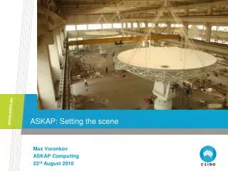
ASKAP: Setting the scene Max Voronkov ASKAP Computing 23rd August 2010
ASKAP overview http://www.atnf.csiro.au/projects/askap/ • Located at radio-quiet site approx. 300 km inland from Geraldton • Array of 36 12m antennas with phased array feeds (PAF) • Initially 6 antennas: BETA (Boolardy Engineering Test Array) • First antenna on site since last year, already used for some science (VLBI with other Australian antennas and Warkworth in New Zealand)
ASKAP 3-axis antenna mount • 3-axis mount allows us to keep beam pattern fixed on the sky
ASKAP: General project news Antennas ahead of schedule BETA antennas (1-6) to arrive to WA within a month Same hardware for beamformer, correlator and tide array unit Digital team redesigned hardware for Virtex 6 FPGA Virtex 7 could be a game changer (direct sampling + 4 boards instead of 32) Ten survey science projects Two high priority projects (EMU,Wallaby) Simulations to ensure software is ready PAF is the main technical risk New technology, fundamentals to learn Aggressive timescale Economical production Performance requirements Scaling is another risk
Calibration & Imaging challenges • Strong sources contaminating the data through primary beam sidelobes • We have 3-axis mount which keeps sidelobes fixed • Beam variations due to PAF instabilities could be a problem • Wide field calibration • Ionosphere is benign at frequencies about 1 GHz • PAF is stabilized in hardware (noise sources) • Software calibration is per synthetic beam • Wide field imaging • Take direction-dependent effects via convolution functions • Wide field deconvolution • Subtraction of the local sky model from uv-data • Joint processing of the full field of view • S/N-based cleaning (eventually MSMF algorithm) CP Applications / Calibration and Imaging
Calibration & Imaging challenges - 2 • Mosaicing in full polarization • Polarisation properties of each beam will be taken care of by adding an extra dimension to convolution functions • Mosaicing with different primary beams • Comes out naturally in our approach to mosaicing (we planned for this up front designing our software, but haven’t tried this case yet in practice) • Large data volumes (LDV) - pipeline processing • Central Processor of ASKAP will reduce data on-the-fly, astronomers are not expected to touch uv-data • Large data volumes (LDV) - data formats • At this stage we use Measurement Sets. In any case, we plan to write a tool exporting the data into MS to assist with debugging (e.g. using casa) CP Applications / Calibration and Imaging
Calibration & Imaging challenges - 3 • Large data volumes (LDV) - processing power limitations and shortcuts (e.g. algorithm and data compression) needed • Shortcuts to ensure single iteration over data is sufficient • Replaced traditional weighting schemes with post-gridding preconditioning (e.g. Wiener filter) • Assumed a good instantaneous uv-coverage • Sky models: greater sophistication in specification • Plan to reuse LOFAR approach • Not much research done so far • Solvability (cal): enough calibrators? • ASKAP field of view has on average 56 Jy of flux • With the target performance figures / 5 min solution interval, it allows to calibrate gain amplitudes with the 2% accuracy and phases with a few degrees accuracy • The impact on the dynamic range is not clear CP Applications / Calibration and Imaging
Calibration & Imaging challenges - 4 • Time and frequency dependence of calibration parameters • Predict forward approach (no interpolation) • Frequency dependence: bandpass, leakages per coarse (1 MHz) channel • Full pol imaging • Specify polarisation of the primary beams via convolution functions (extra dimansions) • On-the-fly mapping (ask Gerry what this means)- Long baselines / large fields of view: dumping fast enough • ASKAP will deliver eventually a continuum map every 5 seconds (for transient search) CP Applications / Calibration and Imaging
Contact Us Phone: 1300 363 400 or +61 3 9545 2176 Email: enquiries@csiro.au Web: www.csiro.au Thank you Australia Telescope National Facility Max Voronkov Software Scientist (ASKAP) Phone: 02 9372 4427 Email: maxim.voronkov@csiro.au Web: http://www.atnf.csiro.au/projects/askap/ CP Applications / Calibration and Imaging