
Enough theory (for now: more to come later!)
Sample Data Analysis: Simple Regression. Enough theory (for now: more to come later!) To look at the data: type cd AFNI_data3/afni ; then afni Switch Underlay to dataset epi_r1 Then Axial Image and Graph FIM Pick Ideal ; then click afni/epi_r1_ideal.1D ; then Set

Enough theory (for now: more to come later!)
E N D
Presentation Transcript
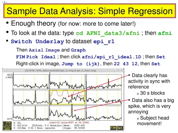
Sample Data Analysis: Simple Regression • Enough theory (for now: more to come later!) • To look at the data: typecd AFNI_data3/afni ; then afni • Switch Underlay to dataset epi_r1 • Then AxialImage and Graph • FIMPick Ideal ; then click afni/epi_r1_ideal.1D ; then Set • Right-click in image, Jump to (ijk), then 22 43 12, then Set • Data clearly has activity in sync with reference • 30 s blocks • Data also has a big spike, which is very annoying • Subject head movement!
Preparing Data for Analysis • Six preparatory steps are common: • Temporal alignment: program 3dtshift • Image registration (AKA realignment): program 3dvolreg • Image smoothing: program 3dmerge • Image masking: program 3dClipLevel or 3dAutomask • Conversion to percentile: programs 3dTstat and 3dcalc • Censoring out time points that are bad: program 3dToutcount or 3dTqual • Not all steps are necessary or desirable in any given case • In this first example, will only do registration, since the data obviously needs this correction
Data Analysis Script • 3dvolreg(3D image registration) will be covered in detail in a later presentation • filename to get estimated motion parameters • 3dDeconvolve = regression code • In file epi_r1_regress: 3dvolreg -base 3 \ -verb \ -prefix epi_r1_reg \ -1Dfile epi_r1_mot.1D \ epi_r1+orig 3dDeconvolve \ -input epi_r1_reg+orig \ -nfirst 3 \ -num_stimts 1 \ -stim_times 1 epi_r1_times.1D \ 'BLOCK(30)' \ -stim_label 1 AllStim \ -tout \ -bucket epi_r1_func \ -fitts epi_r1_fitts \ -xjpeg epi_r1_Xmat.jpg \ -x1D epi_r1_Xmat.x1D • Name of input dataset (from 3dvolreg) • Index of first sub-brick to process [skipping #0-2] • Number of input model time series • Name of input stimulus class timing file (’s) • and type of HRF model to fit • Name for results in AFNI menus • Indicates to output t-statistic for weights • Name of output “bucket” dataset (statistics) • Name of output model fit dataset • Name of image file to store X[AKA R] matrix • Name of text file in which to store X matrix • Type tcsh epi_r1_regress ; then wait for programs to run
} MatrixQuality Assurance • 3dvolreg output • ++ 3dvolreg: AFNI version=AFNI_2007_05_29_1644 (Sep 5 2007) [64-bit] • ++ Reading input dataset ./epi_r1+orig.BRIK • ++ Edging: x=3 y=3 z=2 • ++ Initializing alignment base • ++ Starting final pass on 67 sub-bricks: 0..1..2..3.. *** ..63..64..65..66.. • ++ CPU time for realignment=5.35 s [=0.0799 s/sub-brick] • ++ Min : roll=-0.103 pitch=-1.594 yaw=-0.038 dS=-0.354 dL=-0.021 dP=-0.191 • ++ Mean: roll=-0.047 pitch=+0.061 yaw=+0.023 dS=+0.006 dL=+0.032 dP=-0.076 • ++ Max : roll=+0.065 pitch=+0.290 yaw=+0.055 dS=+0.050 dL=+0.120 dP=+0.113 • ++ Max displacement in automask = 2.46 (mm) at sub-brick 42 • ++ Wrote dataset to disk in ./epi_r1_reg+orig.BRIK • 3dDeconvolve output • ++3dDeconvolve: AFNI version=AFNI_2007_05_29_1644 (Sep 5 2007) [64-bit] • ++ Authored by: B. Douglas Ward, et al. • ++ loading dataset epi_r1_reg+orig • *+ WARNING: Input polort=1; Longest run=201.0 s; Recommended minimum polort=2 • ++ -stim_times using TR=3 seconds • ++ '-stim_times 1' using LOCAL times • ++ Wrote matrix image to file epi_r1_Xmat.jpg • ++ Wrote matrix values to file epi_r1_Xmat.x1D • ++ Signal+Baseline matrix condition [X] (64x3): 2.59165 ++ VERY GOOD ++ • ++ Signal-only matrix condition [X] (64x1): 1 ++ VERY GOOD ++ • ++ Baseline-only matrix condition [X] (64x2): 1.08449 ++ VERY GOOD ++ • ++ -polort-only matrix condition [X] (64x2): 1.08449 ++ VERY GOOD ++ • ++ Matrix inverse average error = 5.62791e-16 ++ VERY GOOD ++ • ++ Calculations starting; elapsed time=0.238 • ++ voxel loop:0123456789.0123456789.0123456789.0123456789.0123456789. • ++ Calculations finished; elapsed time=1.417 • ++ Wrote bucket dataset into ./epi_r1_func+orig.BRIK • ++ Wrote 3D+time dataset into ./epi_r1_fitts+orig.BRIK • ++ #Flops=3.11955e+08 Average Dot Product=4.50251 • If a program crashes, we’ll need to see this text output (at the very least)! Text Output of the epi_r1_decon script }Maximum movement estimate } Consider '-polort 2' }Output file indicators }Progress meter/pacifier }Output file indicators
Stimulus Timing: Input and Visualization X matrix columns epi_r1_times.1D=9.0 69.0 129.0 =times of start of each BLOCK(20) • HRFtiming • Linear in t • All ones epi_r1_Xmat.jpg 1dplot -sepscl epi_r1_Xmat.x1D
Look at the Activation Map • Run afni to view what we’ve got (note: a subtle test over only 1 run) • Switch Underlay to epi_r1_reg (output from 3dvolreg) • Switch Overlay to epi_r1_func (output from 3dDeconvolve) • Sagittal Image and Graph viewers • FIMIgnore3 to have graph viewer not plot 1st 3 time pts • FIMPick Ideal ; pick epi_r1_ideal.1D (output from waver) • Define Overlay to set up functional coloring • OlayAllstim[0] Coef (sets coloring to be from model fit ) • ThrAllstim[0] t-s (sets threshold to be model fit t-statistic) • See Overlay (otherwise won’t see the function!) • Play with threshold slider to get a meaningful activation map (e.g., t =3 is a decent threshold — more on thresholds later) • Again, use Jump to (i j k) to jump to index coordinates 22 43 12
More Looking at the Results • Graph viewer: OptTran 1DDataset #N to plot the model fit dataset output by 3dDeconvolve • Will open the control panel for the Dataset #N plugin • Click first Input on ; then choose Dataset epi_r1_fitts+orig • Also choose Color dk-blue to get a pleasing plot • Then click on Set+Close(to close the plugin’s control panel) • Should now see fitted time series in the graph viewer instead of data time series • Graph viewer: click OptDouble PlotOverlay on to make the fitted time series appear as an overlay curve • This tool lets you visualize the quality of the data fit • Can also now overlay function on MP-RAGE anatomical by using Switch Underlay to anat+orig dataset • Probably won’t want to graph the anat+orig dataset!
Setting the Threshold: Principles • Bad things (i.e., errors): • False positives — activations reported that aren’t really there Type I errors (i.e., activations from noise-only data) • False negatives — non-activations reported where there should be true activations found Type II errors • Usual approach in statistical testing is to control the probability of a type I error (the “p-value”) • In FMRI, we are making many statistical tests: one per voxel (20,000+) — the result of which is an “activation map”: • Voxels are colorized if they survive the statistical thresholding process Start of Important Aside
Setting the Threshold: Bonferroni • If we set the threshold so there is a 1% chance that any given voxel is declared “active” even if its data is pure noise (FMRI jargon: “uncorrected” p-value is 0.01): • And assume each voxel’s noise is independent of its neighbors (not really true) • With 20,000 voxels to threshold, would expect to get 200 false positives — this may be as many as the true activations! Situation: Not so good. • Bonferroni solution: set threshold (e.g., on t-statistic) so high that uncorrected p-value is 0.05/20000=2.5e-6 • Then have only a 5% chance that even a single false positive voxel will be reported • Objection: will likely lose weak areas of activation Important Aside
Setting the Threshold: Spatial Clustering • Cluster-based detection lets us lower the statistical threshold and still control the false positive rate • Two thresholds: • First: a per-voxel threshold that is somewhat low (so by itself leads to a lot of false positives, scattered around) • Second: form clusters of spatially contiguous (neighboring) voxels that survive the first threshold, and keep only those clusters above a volume threshold — e.g., we don’t keep isolated “active” voxels • Usually: choose volume threshold, then calculate voxel-wise statistic threshold to get the overall “corrected” p-value you want (typically, corrected p=0.05) • No easy formulas for this type of dual thresholding, so must use simulation: AFNI program AlphaSim Important Aside
AlphaSim: Clustering Thresholds • Simulated for brain mask of 18,465 voxels • Look for smallest cluster with corrected p < 0.05 Uncorrected p-value (per voxel) 0.0002 0.0004 0.0007 0.0010 0.0020 0.0030 0.0040 0.0050 0.0060 0.0070 0.0080 0.0090 0.0100 Cluster Size / Corrected p (uncorrelated) 2 / 0.001 2 / 0.008 2 / 0.026 3 / 0.001 3 / 0.003 3 / 0.008 3 / 0.018 3 / 0.030 4 / 0.003 4 / 0.004 4 / 0.006 4 / 0.010 4 / 0.015 Cluster Size / Corrected p (correlated 5 mm) 3 / 0.004 4 / 0.012 3 / 0.031 4 / 0.007 4 / 0.032 5 / 0.013 5 / 0.029 6 / 0.012 6 / 0.023 6 / 0.036 7 / 0.016 7 / 0.027 7 / 0.042 Corresponds to sample data Can make activation maps for display with cluster editing using 3dmerge program or in AFNI GUI (new: Sep 2006) End of Important Aside
Multiple Stimulus Classes • The experiment analyzed here in fact is more complicated • There are 9 related communication stimulus types in a 3x3 design of Category by Affect (stimuli are shown to subject as pictures) • Telephone, Email & Face-to-face = categories • Negative, Positive & Neutral = affects • telephone stimuli: tneg, tpos, tneu • email stimuli: eneg, epos, eneu • face-to-face stimuli: fneg, fpos, fneu • Each stimulus type has 3 presentation blocks of 30 s duration • Scrambled pictures are shown between blocks • 9 imaging runs, 64 useful time points in each • Originally, 67 TRs per run, but skip first 3 for MRI signal to reach steady state • So 576 TRs of data, in total • Already registered and put together into dataset rall_vr+orig
Regression with Multiple Model Files • Script file rall_decon does the job: • Run this script by typing tcsh rall_decon (takes a few minutes) 3dDeconvolve -input rall_vr+orig \ -jobs 2 \ -concat '1D: 0 64 128 192 256 320 384 448 512' \ -num_stimts 15 \ -stim_times 1 '1D: 0 * | | | 120 | | | | | 60' 'BLOCK(30)' \ -stim_times 2 '1D: * * || 120 | | 0 | | | | 120' 'BLOCK(30)' \ -stim_times 3 '1D: * * | 120 | | 60 | | | | | 0' 'BLOCK(30)' \ -stim_times 4 '1D: 60 * | | | | | 120 | 0 | |' 'BLOCK(30)' \ -stim_times 5 '1D: * * | 60 | | 0 | | | 120 | |' 'BLOCK(30)' \ -stim_times 6 '1D: * * | | 0 | | 60 | | | 60 |' 'BLOCK(30)' \ -stim_times 7 '1D: * * | 0 | | | 120 | | 60 | |' 'BLOCK(30)' \ -stim_times 8 '1D: 120 * | | | | | 60 | | 0 |' 'BLOCK(30)' \ -stim_times 9 '1D: * * | | 60 | | | 0 | | 120 |' 'BLOCK(30)' \ -stim_label 1 tneg -stim_label 2 tpos -stim_label 3 tneu \ -stim_label 4 eneg -stim_label 5 epos -stim_label 6 eneu \ -stim_label 7 fneg -stim_label 8 fpos -stim_label 9 fneu \ • try to use 2 CPUs • run indices • stimulus times • '|' indicates new run • response model • stimulus label continued…
Regression with Multiple Model Files (continued) • motion regressor • apply to baseline -stim_file 10 motion.1D'[0]' -stim_base 10 \ -stim_file 11 motion.1D'[1]' -stim_base 11 \ -stim_file 12 motion.1D'[2]' -stim_base 12 \ -stim_file 13 motion.1D'[3]' -stim_base 13 \ -stim_file 14 motion.1D'[4]' -stim_base 14 \ -stim_file 15 motion.1D'[5]' -stim_base 15 \ -gltsym 'SYM: tpos -epos' -glt_label 1 TPvsEP \ -gltsym 'SYM: tpos -tneg' -glt_label 2 TPvsTNg \ -gltsym 'SYM: tpos tneu tneg -epos -eneu -eneg' \ -glt_label 3 TvsE \ -fout -tout \ -bucket rall_func -fitts rall_fitts \ -xjpeg rall_xmat.jpg -x1D rall_xmat.x1D • symbolic GLT • label the GLT • statistic types to output • the 9 visual stimulus classes were given using -stim_times • it is important to include motion parameters as regressors • this helps to exclude stimulus correlated motion artifacts • the 6 motion parameters were given using -stim_file • 3dvolreg has previously been run, with the -1Dfile option
} } Regressor Matrix for This Script (via -xjpeg) } Visual stimuli Baseline Motion • 18 baseline regressors • linear baseline • 9 runs times 2 params • 9 visual stimulus regressors • 3x3 stimulus design • 6 motion regressors • 3 shifts, 3 rotations
Regressor Matrix for This Script (via -x1D) baseline regressors: via 1dplot -sepscl xmat_rall.x1D'[0..18]'
Regressor Matrix for This Script(via -x1D) • motion regressors • visual stimuli 1dplot -sepscl xmat_rall.x1D'[18..$]'
Novel Features of 3dDeconvolve - 1 -concat '1D: 0 64 128 192 256 320 384 448 512' • “File” that indicates where distinct imaging runs start inside the input file • Numbers are the time indexes inside the file for start of runs • In this case, a .1D file put directly on the command line • Could also be a filename, if you want to store that data externally -num_stimts 15 • We have 9 visual stimuli (+6 motion), so will need 9 -stim_times below -stim_times 1 '1D: 0.0 * | | | 120.0 | | | | | 60.0' 'BLOCK(20,1)’ • “File” with 9 lines, each line specifying the start time in seconds for the stimuli within the corresponding imaging run, with the time measured relative to the start of the imaging run itself • HRF for each block stimulus is now specified to go to maximum value of 1 (compare to graphs on previous slide) • This feature is useful when converting FMRI response magnitude to be in units of percent of the mean
Aside: the 'BLOCK()' HRF Model • BLOCK(L) is convolution of square wave of duration L with “gamma variate function” (peak value=1 at t=4): • “Hidden” option: BLOCK5 replaces “4” with “5” in the above • Slightly more delayed rise and fall times • BLOCK(L,1) makes peak amplitude of block response=1 Black=BLOCK(20,1) Red=BLOCK5(20,1)
Novel Features of 3dDeconvolve - 2 -gltsym 'SYM: tpos -epos' -glt_label 1 TPvsEP • GLTs are General Linear Tests • 3dDeconvolve provides test statistics for each regressor and stimulus class separately, but if you want to test combinations or contrasts of the weights in each voxel, you need the -gltsym option • Example above tests the difference between the weights for the Positive Telephone and the Positive Emailresponses • Starting with SYM: means symbolic input is on command line • Otherwise inputs will be read from a file • Symbolic names for each stimulus class are taken from -stim_label options • Stimulus label can be preceded by + or - to indicate sign to use in combination of weights • Goal is to test a linear combination of the weights • Tests if tpos– epos=0 • e.g., does tpos get a bigger response than epos ? • Quiz: what would 'SYM: tpos epos' test? It would test if tpos+ epos = 0
Novel Features of 3dDeconvolve - 3 -gltsym 'SYM: tpos tneu tneg -epos -eneu -eneg' -glt_label 3 TvsE • Goal is to test if (tpos + tneu + tneg)–(epos + eneu + eneg)= 0 • Regions where this statistic is significant have different amounts of (average) BOLD signal change in the telephone tasks versus the email tasks • -glt_label 3 TvsEoption is used to attach a meaningful label to the resulting statistics sub-bricks • Output includes the ordered summation of the weights and the associated statistical parameters (t- and/or F-statistics)
Novel Features of 3dDeconvolve - 4 -fout -tout = output both F- and t-statistics for each stimulus class (-fout) and stimulus coefficient (-tout)— but not for the baseline coefficients (if you want baseline statistics: -bout) • The full model statistic is an F-statistic that shows how well the sum of all 9 input model time series fits voxel time series data • Compared to how well just the baseline model time series fit the data times (in this example, have 24 baseline regressor columns in the matrix — 18 for the linear baseline, plus 6 for motion regressors) • The individual stimulus classes also will get individual F- and/or t-statistics indicating the significance of their individual incremental contributions to the data time series fit • e.g.,Ftpos tells if the full model explains more of the data variability than the model with tpos omitted and all other model components included
Results of rall_regress Script • Images showing results from third GLT contrast: ATvsHL • Menu showing labels from 3dDeconvolve run • Play with these results yourself!
Statistics from 3dDeconvolve • An F-statistic measures significance of how much a model component (stimulus class) reduced the variance (sum of squares) of data time series residual • After all the other model components were given their chance to reduce the variance • Residuals data – model fit = errors = -errts • A t-statistic sub-brick measures impact of one coefficient (of course, BLOCK has only one coefficient) • Full F measures how much the all signal regressors combined reduced the variance over just the baseline regressors (sub-brick #0) • Individual partial-model Fs measures how much each individual signal regressor reduced data variance over the full model with that regressor excluded (e.g., sub-bricks #3, #6, #9) • The Coef sub-bricks are the weights (e.g., #1, #4, #7, #10) for the individual regressors • Also present: GLT coefficients and statistics Group Analysis: will be carried out on or GLT coefs from single-subject analyses