Download
1 / 69
760 likes | 1.01k Views
Modelling and Design of the Electrochemical. Processes and Reactors. Karel Bouzek, Roman Kodým. Department of Inorganic Technology,. Institute of Chemical Technology Prague. Mathematical modelling and process design. Role of the mathematical modelling in the electrochemical engineering.

E N D
Modelling and Design of the Electrochemical Processes and Reactors Karel Bouzek, Roman Kodým Department of Inorganic Technology, Institute of Chemical Technology Prague
Mathematical modelling and process design Role of the mathematical modelling in the electrochemical engineering pedagogical deep understanding of the process identification of the rate determining steps learning the way of sequential thinking scientific analysis of the problem on the local scale based on the global experimental data evaluation of not directly accessible parameters verification of the theories developed economical process scale-up process optimisation identification of the possible bottlenecks costs reduction
Mathematical modelling and process design Levels of the mathematical modelling material balance based on the macroscopic kinetics data based on the two elementary modes of operation assessment of the system limits under given assumptions steady state models detail description of the space distribution of the process parameters in steady state allows evaluation of the construction and operational parameters suitability sufficient for the majority of cases dynamic models description of the non-stationary processes process start-up and termination discontinuous processes most sophisticated problems
Mathematical modelling and process design Material balance modes of operation batch (discontinuous) processes continuous processes continuously stirred tank reactor (CSTR) plug-flow reactor (PFR) Batch processes basic characteristics processes in a closed systems (no mass exchange with the surroundings) no steady state is reached before the reaction equilibrium suitable mainly for the small scale processes typical design - stirred tank reactor description by the dynamic model only
Mathematical modelling and process design Batch processes material balance high mixing rate – spatially uniform concentration mass transfer limited reaction concentration decay of component A in time galvanostatic process at j < jlim galvanostatic process at j jlim
Mathematical modelling and process design Continuous process - CSTR material balance high mixing rate – spatially uniform concentration equal inlet and outlet flow rates independent on time – – constant reactor volume and mean residence time concentration decay of component A in time galvanostatic process at j < jlim galvanostatic process at j jlim
Mathematical modelling and process design Continuous process - PFR material balance negligible axial electrolyte mixing negligible concentration gradient perpendicular to the flow direction b – electrode width concentration decay of component A in time galvanostatic process at j < jlim galvanostatic process at j jlim
Steady state models Background of the electrochemical reactors modelling basic parameters calculated local values of the Galvani potential local current density values way of the system description differential or partial differential equations division of the mathematical models according to the level of simplification primary current density distribution secondary current density distribution tertiary current density distribution according to the number of dimensions considered one dimensional two dimensional three dimensional according to the mathematical methods used analytical numerical
Steady state models Level of simplification primary current density distribution infinitely fast reaction kinetics infinitely fast mass transfer kinetics only influencing factors geometry of the system electrolyte conductivity secondary current density distribution reaction kinetics considered more regular current density distribution sufficient approximation for the majority of the industrially relevant systems tertiary current density distribution mass transfer kinetics and electrolyte hydrodynamics considered additional reduction of the local extremes extremely complicated – used only in a strictly limited number of cases
Steady state models Number of dimensions considered selection criteria homogeneity of the system significance of the local irregularities symmetry of the system consequences of the increase in the number of dimensions one-dimensional model described by the differential equations more dimensions requires partial differential equations significantly more complicated mathematics geometrically increasing hardware demands three dimensional models simplified models mainly focus on the critical element of the complex system important mainly in the tertiary current distribution models
Steady state models Mathematical methods used analytical solution of the model equations most accurate way general validity of the equations derived (for the given system) available for the extremely simple configurations only strongly limited applicability in the industrially relevant systems numerical mathematics able to describe complicated geometries and complex systems less significant simplification assumptions results valid only for the particular system solved question of results accuracy methods of numerical mathematics used strongly dependent on the dimensions number one dimensional case - classical integration methods (Runge-Kutta, collocation, shooting, …) more dimensional tasks – rapid development with improving hardware FDM FEM BEM
Steady state models Basic model equations for electrochemical systems equation of the mass and charge transfer in the electrolyte solution Nernst-Planck equation current density value application of the Faraday law electroneutrality condition electrolyte solution with no concentration gradients electrolyte conductivity definition
Steady state models Basic model equations for electrochemical systems electrolyte solution with concentration gradients current less system liquid junction potential one dimensional case
Steady state models Basic model equations for electrochemical systems mass balance in the electrolyte volume introducing Nernts-Planck equation after multiplication by ziF electroneutrality condition charge conservation no concentration gradients introducing expression for j Laplace equation modified Laplace equation
Steady state models Boundary conditions significant variability according to the particular conditions in agreement with general types of boundary conditions constant value, i.e. Galvani potential constant flux, i.e. current density Boundary condition – constant potential value arbitrary definition requirements: no influence of the current load constant composition, i.e. constant properties typical choices: electrode current leads potentials electrode body potential arbitrary values typically used: cathode – potential equal to zero anode – potential equal to the cell voltage special case – electrode / electrolyte interface
Steady state models Boundary condition – constant flux typically the cell walls and electrolyte surface (no flux) in special cases flux continuity used Electrode / electrolyte interface simplification considered: primary vs. secondary (tertiary) current density distribution potential rate determining steps in the electrode reaction kinetics kinetics of the mass transfer to the electrode adsorption charge transfer kinetics desorption of the products kinetics of the product transfer from the electrode possible homogeneous reactions mass transfer kinetics subject of the individual lecture types of the charge transfer kinetics used: linear Tafel Butler-Volmer
Steady state models Linear kinetics historical question computational demands physical models nowadays overcome Tafel kinetics considers just one part of the polarisation curve suitable for the systems far from equilibrium simple kinetics evaluation from the model results linearisation of the low current densities part - - minimisation of the divergence danger
Steady state models Butler - Volmer kinetics general description of the charge transfer kinetics more complicated kinetic evaluation (requires additional numerical procedure) mass transfer limited kinetics - concentration polarisation charge transfer limited kinetics
Steady state models Classical approach – finite differences first detail models of the electrochemical reactors transformation of the partial differential equation to the set of linear equations Taylor's expansion used for linearisation symmetrical formulas for the first and second derivative
Steady state models Classical approach – finite differences asymmetrical formulas – boundary conditions
Steady state models Classical approach – finite differences method of replacement of the partial derivatives in the Laplace equation principle of the Laplace equation divergence of the flux equal to zero etc.
Steady state models Classical approach – finite differences flux divergence in the final differences
Finite differences example Current density simulation in the parallel plate cell current density distribution in the zinc electrowinning cell K. Bouzek, K. Borve, O.A. Lorentsen, K. Osmudsen, I. Roušar, J. Thonstad, J. Electrochem. Soc.142 (1995) 64.
Finite differences example Current density simulation in the parallel plate cell current density distribution in the zinc electrowinning cell K. Bouzek, K. Borve, O.A. Lorentsen, K. Osmudsen, I. Roušar, J. Thonstad, J. Electrochem. Soc.142 (1995) 64.
Steady state models Classical approach – finite differences FDM applicable for solving of any type of partial differential equation complications may be expected in the case of complex boundary conditions form slow convergence problems often related to the anistropic media difficulties by solving systems with the irregular geometries alternative approaches searched
Steady state models Recent approach – finite element method (FEM) original approach based on the calculus of variations doesn’t solve the equation directly (approximation method) searching for the function giving extreme by replacing the differential equation such function approximated by a sum of the basis functions (unknown coefficients) coefficients determined by solving a system of linear algebraic equations drawbacks largely depends on the choice of the basis functions cannot be satisfied for too complicated geometries finite elements method the function is not searched for the whole domain integrated domain is divided into the a number of subdomains in each subdomain solution approximated by a simple function Galerkin’s method of weighted residuals, i.e. parameters of the basis function modifications maybe derived by the choice of the weighting functions necessary condition is that the combination of basis functions fulfil boundary conditions
Steady state models Recent approach – finite element method (FEM) application onto the solution of the Laplace equation approximate expression by the means of FEM simplification for the one-dimensional case approximate expression takes following form FEM is optimising value of ui in such a way, that is close to 0
ji(x) 1 x 0 x0 x1 xi-1 xi xi+1 xN-1 xN Steady state models Recent approach – finite element method (FEM) simplest linear basis function
Examples of the FEM applications Parametric study of the narrow gap cell current density distribution in the channel with parallel plate electrodes
Examples of the FEM applications Curved boundary presence of the gas bubble in the interelectrode space
Examples of the FEM applications Optimisation of the direct electrochemical water disinfection cell evaluation of the process efficiency 2.4 cm 5 cm 0.3 cm 0.5 cm 10 cm A C A C 5 cm y x
Examples of the FEM applications Optimisation of the direct electrochemical water disinfection cell evaluation of the process efficiency – plate electrodes anode cathode anode U = 6.04 V Javer.= 50 A m-2 s= 667 mS cm-1 = 4.92 %
Examples of the FEM applications Optimisation of the direct electrochemical water disinfection cell evaluation of the process efficiency – plate electrodes U = 6.04 V Javer.= 50 A m-2 s= 667 mS cm-1 = 4.92 %
z x y Examples of the FEM applications Optimisation of the direct electrochemical water disinfection cell evaluation of the process efficiency – expanded mesh electrodes cathode 3 mm anode 1.5 mm 5 mm 1.4 mm
Examples of the FEM applications Optimisation of the direct electrochemical water disinfection cell evaluation of the process efficiency – expanded mesh electrodes U = 4.76 V Javer.= 42.4 A m-2 s= 667 mS cm-1 = 4.12 %
Finite volumes method Alternative to FEM handling flux densities principle of the method solution of partial differential eqs. based on the PDE integration ( i-1, j+1 ) ( i , j+1 ) ( i+1, j+1 ) over the volume surrounding controlled grid point controlled domain covered by the controlled volumes integration leads formally to equation identical with FDE ( i-1, j ) ( i , j ) ( i+1, j ) ( i , j-1 ) ( i-1, j-1 ) ( i+1, j-1 )
Finite volumes method Application to the bipolar electrode function simulation model system under study Terminal Cathode Terminal Anode Electrolyte 14 1.5 Bipolar Pt electrode [mm] 780 55 Cylindrical coordinate system r - radius r x – position x
Finite volumes method Application to the bipolar electrode function simulation model system under study I = 40 mA; U =4 V
Finite volumes method Application to the bipolar electrode function simulation model system under study I = 40 mA; U =4 V
Finite volumes method Application to the bipolar electrode function simulation comparison of the model and experimental results
Tertiary current density distribution Potential and current density distribution in three dimensional electrode model system under study
Tertiary current density distribution Potential and current density distribution in three dimensional electrode simplified sketch of the cell construction 1 – electrolyte inlet 5 – anode feeder 6 – anode 2 – particle electrode 7 – separator 3 – channels connecting individual drums 8 – electrolyte outlet 4 – cathode feeder
Tertiary current density distribution Potential and current density distribution in three dimensional electrode simplified flow patterns inside the cell - electrolyte
Tertiary current density distribution Potential and current density distribution in three dimensional electrode simplified flow patterns inside the cell – electric current
Tertiary current density distribution Potential and current density distribution in three dimensional electrode basic equations describing the system Nomenclature jm – Galvani potential of the electrode phase js – Galvani potential of the electrolyte phase electrode phase km – conductivity of the electrode phase ks – conductivity of the electrolyte phase ae – electrode spec. surface jel– current density corresponding to the electrode reaction electrolyte phase x – coordinate
Tertiary current density distribution Potential and current density distribution in three dimensional electrode basic equations describing the system – definition of jel electrode reactions considered: Cu cathode Cu2+ + 2e- H2 2 H+ + 2e- 4 H+ + O2 anode 2 H2O overall electrode reaction current density: resistivity to the charge transfer:electrode potential
Tertiary current density distribution Potential and current density distribution in three dimensional electrode basic equations describing the system – electrode reaction kinetics
Tertiary current density distribution Potential and current density distribution in three dimensional electrode basic equations describing the system – electrode reaction kinetics polarisation curves reversible potentials: Nernst equation
Tertiary current density distribution Potential and current density distribution in three dimensional electrode basic equations describing the system – electrode reaction kinetics mass transfer coefficient evaluation significant complication – evaluation of the linear electrolyte flow rate
Tertiary current density distribution Potential and current density distribution in three dimensional electrode selected results – influence of the current load cCu0 = 7.87 mol m-3 V = 4.5·10-5 m3 s-1 k = 4.19·10-6 m s-1 cH0 = 100 mol m-3 particle diameter 0.002 m w = 0.047 Hz