Download
1 / 53
610 likes | 892 Views
a. . AQL LTPD. Supplement J - Acceptance Sampling Plans. Sequential Sampling Chart. 8 – 7 – 6 – 5 – 4 – 3 – 2 – 1 – 0 –. Number of defectives. | | | | | | | 10 20 30 40 50 60 70. Cumulative sample size. Figure J.1. Sequential Sampling Chart. 8 – 7 –

E N D
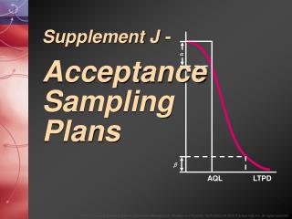
a AQL LTPD Supplement J -Acceptance SamplingPlans
8 – 7 – 6 – 5 – 4 – 3 – 2 – 1 – 0 – Number of defectives | | | | | | | 10 20 30 40 50 60 70 Cumulative sample size Figure J.1 Sequential Sampling Chart
8 – 7 – 6 – 5 – 4 – 3 – 2 – 1 – 0 – Number of defectives Continue sampling | | | | | | | 10 20 30 40 50 60 70 Cumulative sample size Figure J.1 Sequential Sampling Chart
8 – 7 – 6 – 5 – 4 – 3 – 2 – 1 – 0 – Reject Number of defectives Continue sampling Accept | | | | | | | 10 20 30 40 50 60 70 Cumulative sample size Figure J.1 Sequential Sampling Chart
8 – 7 – 6 – 5 – 4 – 3 – 2 – 1 – 0 – Decision to reject Reject Number of defectives Continue sampling Accept | | | | | | | 10 20 30 40 50 60 70 Cumulative sample size Figure J.1 Sequential Sampling Chart
Probability of acceptance Proportion defective Figure J.2 Operating Characteristic Curve
Ideal OC curve Probability of acceptance Proportion defective Figure J.2 Operating Characteristic Curve
Ideal OC curve Probability of acceptance Typical OC curve Proportion defective Figure J.2 Operating Characteristic Curve
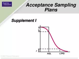
1.0 Ideal OC curve a Probability of acceptance Typical OC curve AQL LTPD Proportion defective Figure J.2 Operating Characteristic Curve
1.0 – 0.9 – 0.8 – 0.7 – 0.6 – 0.5 – 0.4 – 0.3 – 0.2 – 0.1 – 0.0 – Probability of acceptance | | | | | | | | | | 1 2 3 4 5 6 7 8 9 10 (AQL) (LTPD) Proportion defective (hundredths) Operating Characteristic Curve Example J.1
1.0 – 0.9 – 0.8 – 0.7 – 0.6 – 0.5 – 0.4 – 0.3 – 0.2 – 0.1 – 0.0 – Probability Proportion of c or less defective defects (p) np (Pa) Comments n = 60 c = 1 Probability of acceptance | | | | | | | | | | 1 2 3 4 5 6 7 8 9 10 (AQL) (LTPD) Proportion defective (hundredths) Operating Characteristic Curve Example J.1
1.0 – 0.9 – 0.8 – 0.7 – 0.6 – 0.5 – 0.4 – 0.3 – 0.2 – 0.1 – 0.0 – np 0 1 2 .05 .951 .999 1.000 .10 .905 .995 1.000 .15 .861 .990 .999 .20 .819 .982 .999 .25 .779 .974 .998 .30 .741 .963 .996 .35 .705 .951 .994 .40 .670 .938 .992 .45 .638 .925 .989 .50 .607 .910 .986 .55 .577 .894 .982 .60 .549 .878 .977 .65 .522 .861 .972 Probability Proportion of c or less defective defects (p) np (Pa) Comments n = 60 c = 1 Probability of acceptance | | | | | | | | | | 1 2 3 4 5 6 7 8 9 10 (AQL) (LTPD) Proportion defective (hundredths) Operating Characteristic Curve Example J.1
1.0 – 0.9 – 0.8 – 0.7 – 0.6 – 0.5 – 0.4 – 0.3 – 0.2 – 0.1 – 0.0 – np 0 1 2 .05 .951 .999 1.000 .10 .905 .995 1.000 .15 .861 .990 .999 .20 .819 .982 .999 .25 .779 .974 .998 .30 .741 .963 .996 .35 .705 .951 .994 .40 .670 .938 .992 .45 .638 .925 .989 .50 .607 .910 .986 .55 .577 .894 .982 .60 .549 .878 .977 .65 .522 .861 .972 Probability Proportion of c or less Defective defects (p) np (Pa) Comments n = 60 c = 1 0.01 (AQL) 0.6 Probability of acceptance | | | | | | | | | | 1 2 3 4 5 6 7 8 9 10 (AQL) (LTPD) Proportion defective (hundredths) Operating Characteristic Curve Example J.1
1.0 – 0.9 – 0.8 – 0.7 – 0.6 – 0.5 – 0.4 – 0.3 – 0.2 – 0.1 – 0.0 – np 0 1 2 .05 .951 .999 1.000 .10 .905 .995 1.000 .15 .861 .990 .999 .20 .819 .982 .999 .25 .779 .974 .998 .30 .741 .963 .996 .35 .705 .951 .994 .40 .670 .938 .992 .45 .638 .925 .989 .50 .607 .910 .986 .55 .577 .894 .982 .60 .549 .878 .977 .65 .522 .861 .972 Probability Proportion of c or less defective defects (p) np (Pa) Comments n = 60 c = 1 0.01 (AQL) 0.6 Probability of acceptance | | | | | | | | | | 1 2 3 4 5 6 7 8 9 10 (AQL) (LTPD) Proportion defective (hundredths) Operating Characteristic Curve Example J.1
1.0 – 0.9 – 0.8 – 0.7 – 0.6 – 0.5 – 0.4 – 0.3 – 0.2 – 0.1 – 0.0 – np 0 1 2 .05 .951 .999 1.000 .10 .905 .995 1.000 .15 .861 .990 .999 .20 .819 .982 .999 .25 .779 .974 .998 .30 .741 .963 .996 .35 .705 .951 .994 .40 .670 .938 .992 .45 .638 .925 .989 .50 .607 .910 .986 .55 .577 .894 .982 .60 .549 .878 .977 .65 .522 .861 .972 Probability Proportion of c or less defective defects (p) np (Pa) Comments n = 60 c = 1 0.01 (AQL) 0.6 0.878 Probability of acceptance | | | | | | | | | | 1 2 3 4 5 6 7 8 9 10 (AQL) (LTPD) Proportion defective (hundredths) Operating Characteristic Curve Example J.1
1.0 – 0.9 – 0.8 – 0.7 – 0.6 – 0.5 – 0.4 – 0.3 – 0.2 – 0.1 – 0.0 – np 0 1 2 .05 .951 .999 1.000 .10 .905 .995 1.000 .15 .861 .990 .999 .20 .819 .982 .999 .25 .779 .974 .998 .30 .741 .963 .996 .35 .705 .951 .994 .40 .670 .938 .992 .45 .638 .925 .989 .50 .607 .910 .986 .55 .577 .894 .982 .60 .549 .878 .977 .65 .522 .861 .972 Probability Proportion of c or less defective defects (p) np (Pa) Comments n = 60 c = 1 0.01 (AQL) 0.6 0.878 Probability of acceptance | | | | | | | | | | 1 2 3 4 5 6 7 8 9 10 (AQL) (LTPD) Proportion defective (hundredths) Operating Characteristic Curve Example J.1
1.0 – 0.9 – 0.8 – 0.7 – 0.6 – 0.5 – 0.4 – 0.3 – 0.2 – 0.1 – 0.0 – Probability Proportion of c or less defective defects (p) np (Pa) Comments n = 60 c = 1 0.01 (AQL) 0.6 0.878 Probability of acceptance | | | | | | | | | | 1 2 3 4 5 6 7 8 9 10 (AQL) (LTPD) Proportion defective (hundredths) Operating Characteristic Curve Example J.1
1.0 – 0.9 – 0.8 – 0.7 – 0.6 – 0.5 – 0.4 – 0.3 – 0.2 – 0.1 – 0.0 – Probability Proportion of c or less defective defects (p) np (Pa) Comments n = 60 c = 1 0.663 0.01 (AQL) 0.6 0.878 a = 1.000 – 0.878 = 0.122 0.02 1.2 0.663 0.03 1.8 0.463 0.04 2.4 0.308 0.05 3.0 0.199 0.06 (LTPD) 3.6 0.126 b = 0.126 0.07 4.2 0.078 0.08 4.8 0.048 0.09 5.4 0.029 0.10 6.0 0.017 Probability of acceptance 0.308 0.199 0.048 | | | | | | | | | | 1 2 3 4 5 6 7 8 9 10 (AQL) (LTPD) Proportion defective (hundredths) Operating Characteristic Curve Example J.1
1.0 – 0.9 – 0.8 – 0.7 – 0.6 – 0.5 – 0.4 – 0.3 – 0.2 – 0.1 – 0.0 – 0.878 0.663 Probability of acceptance 0.463 0.308 0.199 0.126 0.078 0.048 0.029 | | | | | | | | | | 1 2 3 4 5 6 7 8 9 10 0.017 (AQL) (LTPD) Proportion defective (hundredths) Operating Characteristic Curve Example J.1
1.0 – 0.9 – 0.8 – 0.7 – 0.6 – 0.5 – 0.4 – 0.3 – 0.2 – 0.1 – 0.0 – a = 0.122 0.878 0.663 Probability of acceptance 0.463 0.308 0.199 0.126 0.078 0.048 0.029 b = 0.126 | | | | | | | | | | 1 2 3 4 5 6 7 8 9 10 0.017 (AQL) (LTPD) Proportion defective (hundredths) Operating Characteristic Curve Figure J.3
Operating Characteristic Curve 1.0 – 0.9 – 0.8 – 0.7 – 0.6 – 0.5 – 0.4 – 0.3 – 0.2 – 0.1 – 0.0 – Probability of acceptance | | | | | | | | | | 1 2 3 4 5 6 7 8 9 10 (AQL) (LTPD) Proportion defective (hundredths) Figure J.4
Producer’s Consumer’s Risk Risk n (p = AQL) (p = LTPD) Operating Characteristic Curve 1.0 – 0.9 – 0.8 – 0.7 – 0.6 – 0.5 – 0.4 – 0.3 – 0.2 – 0.1 – 0.0 – Probability of acceptance | | | | | | | | | | 1 2 3 4 5 6 7 8 9 10 (AQL) (LTPD) Proportion defective (hundredths) Figure J.4
Producer’s Consumer’s Risk Risk n (p = AQL) (p = LTPD) 60 0.122 0.126 Operating Characteristic Curve 1.0 – 0.9 – 0.8 – 0.7 – 0.6 – 0.5 – 0.4 – 0.3 – 0.2 – 0.1 – 0.0 – Probability of acceptance | | | | | | | | | | 1 2 3 4 5 6 7 8 9 10 (AQL) (LTPD) Proportion defective (hundredths) Figure J.4
Producer’s Consumer’s Risk Risk n (p = AQL) (p = LTPD) 60 0.122 0.126 80 0.191 0.048 Operating Characteristic Curve 1.0 – 0.9 – 0.8 – 0.7 – 0.6 – 0.5 – 0.4 – 0.3 – 0.2 – 0.1 – 0.0 – Probability of acceptance | | | | | | | | | | 1 2 3 4 5 6 7 8 9 10 (AQL) (LTPD) Proportion defective (hundredths) Figure J.4
Producer’s Consumer’s Risk Risk n (p = AQL) (p = LTPD) 60 0.122 0.126 80 0.191 0.048 100 0.264 0.017 Operating Characteristic Curve 1.0 – 0.9 – 0.8 – 0.7 – 0.6 – 0.5 – 0.4 – 0.3 – 0.2 – 0.1 – 0.0 – Probability of acceptance | | | | | | | | | | 1 2 3 4 5 6 7 8 9 10 (AQL) (LTPD) Proportion defective (hundredths) Figure J.4
Producer’s Consumer’s Risk Risk n (p = AQL) (p = LTPD) 60 0.122 0.126 80 0.191 0.048 100 0.264 0.017 120 0.332 0.006 Operating Characteristic Curve 1.0 – 0.9 – 0.8 – 0.7 – 0.6 – 0.5 – 0.4 – 0.3 – 0.2 – 0.1 – 0.0 – Probability of acceptance | | | | | | | | | | 1 2 3 4 5 6 7 8 9 10 (AQL) (LTPD) Proportion defective (hundredths) Figure J.4
Operating Characteristic Curve 1.0 – 0.9 – 0.8 – 0.7 – 0.6 – 0.5 – 0.4 – 0.3 – 0.2 – 0.1 – 0.0 – n = 60, c = 1 n = 80, c = 1 n = 100, c = 1 Probability of acceptance n = 120, c = 1 | | | | | | | | | | 1 2 3 4 5 6 7 8 9 10 (AQL) (LTPD) Proportion defective (hundredths) Figure J.4
Operating Characteristic Curve 1.0 – 0.9 – 0.8 – 0.7 – 0.6 – 0.5 – 0.4 – 0.3 – 0.2 – 0.1 – 0.0 – Probability of acceptance | | | | | | | | | | 1 2 3 4 5 6 7 8 9 10 (AQL) (LTPD) Proportion defective (hundredths) Figure J.5
Producer’s Consumer’s Risk Risk c (p = AQL) (p = LTPD) Operating Characteristic Curve 1.0 – 0.9 – 0.8 – 0.7 – 0.6 – 0.5 – 0.4 – 0.3 – 0.2 – 0.1 – 0.0 – Probability of acceptance | | | | | | | | | | 1 2 3 4 5 6 7 8 9 10 (AQL) (LTPD) Proportion defective (hundredths) Figure J.5
Producer’s Consumer’s Risk Risk c (p = AQL) (p = LTPD) 1 0.122 0.126 Operating Characteristic Curve 1.0 – 0.9 – 0.8 – 0.7 – 0.6 – 0.5 – 0.4 – 0.3 – 0.2 – 0.1 – 0.0 – Probability of acceptance | | | | | | | | | | 1 2 3 4 5 6 7 8 9 10 (AQL) (LTPD) Proportion defective (hundredths) Figure J.5
Producer’s Consumer’s Risk Risk c (p = AQL) (p = LTPD) 1 0.122 0.126 2 0.023 0.303 Operating Characteristic Curve 1.0 – 0.9 – 0.8 – 0.7 – 0.6 – 0.5 – 0.4 – 0.3 – 0.2 – 0.1 – 0.0 – Probability of acceptance | | | | | | | | | | 1 2 3 4 5 6 7 8 9 10 (AQL) (LTPD) Proportion defective (hundredths) Figure J.5
Producer’s Consumer’s Risk Risk c (p = AQL) (p = LTPD) 1 0.122 0.126 2 0.023 0.303 3 0.003 0.515 Operating Characteristic Curve 1.0 – 0.9 – 0.8 – 0.7 – 0.6 – 0.5 – 0.4 – 0.3 – 0.2 – 0.1 – 0.0 – Probability of acceptance | | | | | | | | | | 1 2 3 4 5 6 7 8 9 10 (AQL) (LTPD) Proportion defective (hundredths) Figure J.5
Producer’s Consumer’s Risk Risk c (p = AQL) (p = LTPD) 1 0.122 0.126 2 0.023 0.303 3 0.003 0.515 4 0.000 0.726 Operating Characteristic Curve 1.0 – 0.9 – 0.8 – 0.7 – 0.6 – 0.5 – 0.4 – 0.3 – 0.2 – 0.1 – 0.0 – Probability of acceptance | | | | | | | | | | 1 2 3 4 5 6 7 8 9 10 (AQL) (LTPD) Proportion defective (hundredths) Figure J.5
Operating Characteristic Curve n = 60, c = 1 1.0 – 0.9 – 0.8 – 0.7 – 0.6 – 0.5 – 0.4 – 0.3 – 0.2 – 0.1 – 0.0 – n = 60, c = 2 n = 60, c = 3 n = 60, c = 4 Probability of acceptance | | | | | | | | | | 1 2 3 4 5 6 7 8 9 10 (AQL) (LTPD) Proportion defective (hundredths) Figure J.5
AQL Based LTPD Based Acceptance Expected Sample Expected Sample Number Defectives Size Defectives Size 0 0.0509 5 2.2996 38 1 0.3552 36 3.8875 65 2 0.8112 81 5.3217 89 3 1.3675 137 6.6697 111 4 1.9680 197 7.9894 133 5 2.6256 263 9.2647 154 6 3.2838 328 10.5139 175 7 3.9794 398 11.7726 196 8 4.6936 469 12.9903 217 9 5.4237 542 14.2042 237 10 6.1635 616 15.4036 257 Acceptance Sampling Plan
1.6 – 1.2 – 0.8 – 0.4 – 0 – Average outgoing quality (percent) | | | | | | | | 1 2 3 4 5 6 7 8 Defectives in lot (percent) Operating Characteristic Curve Example J.2
1.6 – 1.2 – 0.8 – 0.4 – 0 – Proportion Probability Defective of Acceptance (p) np (Pa) Average outgoing quality (percent) | | | | | | | | 1 2 3 4 5 6 7 8 Defectives in lot (percent) Operating Characteristic Curve Example J.2
1.6 – 1.2 – 0.8 – 0.4 – 0 – Proportion Probability Defective of Acceptance (p) np (Pa) 0.01 1.10 0.974 0.02 2.20 0.819 0.03 3.30 0.581 = (0.603 + 0.558)/2 0.04 4.40 0.359 0.05 5.50 0.202 = (0.213 + 0.191)/2 0.06 6.60 0.105 0.07 7.70 0.052 = (0.055 + 0.048)/2 0.08 8.80 0.024 Average outgoing quality (percent) | | | | | | | | 1 2 3 4 5 6 7 8 Defectives in lot (percent) Operating Characteristic Curve Example J.2
1.6 – 1.2 – 0.8 – 0.4 – 0 – Proportion Probability Defective of Acceptance (p) np (Pa) 0.01 1.10 0.974 0.02 2.20 0.819 0.03 3.30 0.581 = (0.603 + 0.558)/2 0.04 4.40 0.359 0.05 5.50 0.202 = (0.213 + 0.191)/2 0.06 6.60 0.105 0.07 7.70 0.052 = (0.055 + 0.048)/2 0.08 8.80 0.024 For p = 0.01: Average outgoing quality (percent) | | | | | | | | 1 2 3 4 5 6 7 8 Defectives in lot (percent) Operating Characteristic Curve Example J.2
1.6 – 1.2 – 0.8 – 0.4 – 0 – Proportion Probability Defective of Acceptance (p) np (Pa) 0.01 1.10 0.974 0.02 2.20 0.819 0.03 3.30 0.581 = (0.603 + 0.558)/2 0.04 4.40 0.359 0.05 5.50 0.202 = (0.213 + 0.191)/2 0.06 6.60 0.105 0.07 7.70 0.052 = (0.055 + 0.048)/2 0.08 8.80 0.024 For p = 0.01: 0.01(0.974)(1000 – 110)/1000 = 0.0087 Average outgoing quality (percent) | | | | | | | | 1 2 3 4 5 6 7 8 Defectives in lot (percent) Operating Characteristic Curve Example J.2
1.6 – 1.2 – 0.8 – 0.4 – 0 – Proportion Probability Defective of Acceptance (p) np (Pa) 0.01 1.10 0.974 0.02 2.20 0.819 0.03 3.30 0.581 = (0.603 + 0.558)/2 0.04 4.40 0.359 0.05 5.50 0.202 = (0.213 + 0.191)/2 0.06 6.60 0.105 0.07 7.70 0.052 = (0.055 + 0.048)/2 0.08 8.80 0.024 For p = 0.01: 0.01(0.974)(1000 – 110)/1000 = 0.0087 Average outgoing quality (percent) | | | | | | | | 1 2 3 4 5 6 7 8 Defectives in lot (percent) Operating Characteristic Curve Example J.2
1.6 – 1.2 – 0.8 – 0.4 – 0 – Proportion Probability Defective of Acceptance (p) np (Pa) 0.01 1.10 0.974 0.02 2.20 0.819 0.03 3.30 0.581 = (0.603 + 0.558)/2 0.04 4.40 0.359 0.05 5.50 0.202 = (0.213 + 0.191)/2 0.06 6.60 0.105 0.07 7.70 0.052 = (0.055 + 0.048)/2 0.08 8.80 0.024 For p = 0.01: 0.01(0.974)(1000 – 110)/1000 = 0.0087 For p = 0.02: 0.02(0.819)(1000 – 110)/1000 = 0.0146 For p = 0.03: 0.03(0.581)(1000 – 110)/1000 = 0.0155 For p = 0.04: 0.04(0.359)(1000 – 110)/1000 = 0.0128 For p = 0.05: 0.05(0.202)(1000 – 110)/1000 = 0.0090 For p = 0.06: 0.06(0.105)(1000 – 110)/1000 = 0.0056 For p = 0.07: 0.07(0.052)(1000 – 110)/1000 = 0.0032 For p = 0.08: 0.08(0.024)(1000 – 110)/1000 = 0.0017 Average outgoing quality (percent) | | | | | | | | 1 2 3 4 5 6 7 8 Defectives in lot (percent) Operating Characteristic Curve Example J.2
1.6 – 1.2 – 0.8 – 0.4 – 0 – Proportion Probability Defective of Acceptance (p) np (Pa) 0.01 1.10 0.974 0.02 2.20 0.819 0.03 3.30 0.581 = (0.603 + 0.558)/2 0.04 4.40 0.359 0.05 5.50 0.202 = (0.213 + 0.191)/2 0.06 6.60 0.105 0.07 7.70 0.052 = (0.055 + 0.048)/2 0.08 8.80 0.024 Average outgoing quality (percent) | | | | | | | | 1 2 3 4 5 6 7 8 Defectives in lot (percent) Operating Characteristic Curve Example J.2