Age
The Schooling Decision. Dollars/year. 40,000. Goes to College. (24,000)(65–22) = $1,032,000 (benefit of education). Quits After High School. 16,000. Age. 0. 18. 22. 65. $20,000. + = $84,000 (total cost of education). $64,000. -5,000.

Age
E N D
Presentation Transcript
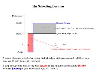
The Schooling Decision Dollars/year 40,000 Goes to College (24,000)(65–22) = $1,032,000 (benefit of education) Quits After High School 16,000 Age 0 18 22 65 $20,000 + = $84,000 (total cost of education) $64,000 -5,000 A person who quits school after getting his high school diploma can earn $16,000 per year from age 18 until the age of retirement. If the person goes to college, she pays $20,000 in tuition and foregoes earning $64,000, but earns $40,000 per year between the ages of 18 and 22. $64,000,
The Schooling Decision • The previous model ignores the discount rate • The higher the discount rate, the less likely someone will invest in education since they are less future oriented • The discount rate depends on: • The market rate of interest • “time preferences” • Swann (2003) estimates the annual discount rate of women at r = 20%
The Schooling Decision • Keane and Wolpin (1997) estimate the discount rate of young men at r = 28% • Do these two results explain why black women graduate • from college at higher rates than black men?
The Schooling Decision • The slope indicates earnings increase in years of education, and the wage-schooling locus in concave • The worker makes $33,600 graduating from JHS • The worker makes $41,600 graduating from HS • The worker makes $46,400 graduating from Univ (41,600-33,600)/33,600 = 23.8% (46,400-41,600)/41,600 =11.5%
The Schooling Decision • The Marginal Rate of Return (to an additional year of schooling) is the percent change in w given a one-year increase in s • Finishing the 8th grade increases earnings by 8% • Finishing 12th grade increases earnings by 4.3% • Finishing college (rather than dropping out after your junior year) increases earnings by 2%
Estimating MRR The Schooling Decision • A typical study estimates a regression of the form: Log(wi) = dxi + asi • wi is the wage rate of the i th worker • si is the years of schooling of the i th worker • In log-linear models, coefficient a represents the • percent increase in w (we took the log of its values) for a • 1 year increase in s (we did not take the log of its values): • Hence a is an estimate for the rate of return to an added year of schooling aMRR
The Schooling Decision r s* • A worker maximizes the present value of lifetime earnings by going to school until the marginal rate of return to schooling equals the discount rate. • A worker with discount rate r = 4.3% goes to school for s* = 12 years.
The Schooling Decision Individuals with different discount rates Rate of Interest Dollars wBS rAl wHS rBob MRR Years of Schooling Years of Schooling 12 12 16 16
The Schooling Decision Individuals with different abilities Rate of Interest Dollars Bob wBob BS Ace wAce wAce r MRRBob MRRAce 12 16 12 16 Years of Schooling Years of Schooling • Ace and Bob have the same discount rate (r) but each worker faces a different wage-schooling locus. • Ace doesn’t go to college since his MRR = r after graduating HS, • Bob graduates from college, and earns wACE. and earns wBOB.
The Schooling Decision Individuals with different abilities Slope is biased Dollars Bob wBob Ace Unbiased slope because ‘ability’ is accounted for in the regression wAce 12 16 Years of Schooling • The wage differential between Bob and Ace arises both because • We don’t observe either wage school locus • Bob goes to school for four more years because • Bob is more able. • As a result, this wage differential does not tells us by how much Ace’s earnings would increase if he were to complete high school.
The Schooling Decision • In studies of twins, presumably holding ability constant, valid estimates of rate of return to schooling can be estimated • Generally, the rate of return to schooling is higher for workers who were born in states with well-funded education systems Source: David Card and Alan B. Krueger, “Does School Quality Matter? Returns to Education and the Characteristics of Public Schools in the United States,” Journal of Political Economy 100 (February 1992), Tables 1 and 2. The data in the graphs refer to the rate of return to school and the school quality variables for the cohort of persons born in 1920-1929.
Education is a Signal • Education reveals a level of attainment which signals a worker’s qualifications to potential employers • Information that is used to allocate a workers in the labor market is called a signal • There could be a “separating equilibrium” • Low-productivity workers choose not to obtain X years of education, voluntarily signaling their low productivity • High-productivity workers choose to get at least X years of schooling and separate themselves from the pack
Education is a Signal Dollars Dollars Costs = 25,001s Costs = 20,000s 100,004 100,000 100,000 80,000 0 0 Years of Schooling Years of Schooling 0 0 4 4 (a)Low-Productivity Workers (b)High-Productivity Workers • Workers get paid $200,000 if they get less than 4 years of college, and $300,000 if they get at least 4 years (Dw = 100,000 if college grad but Dw = 0 if not). • Low-productivity workers find it expensive to invest in college and choose Dw = 0 and s = 0 • High-productivity workers find it inexpensive to invest in college and choose Dw = 100,000 and s = 4 • As a result, the worker’s education signals if he is a low-productivity or a high-productivity worker.
Education is an Investment in Human Capital Men • Highly educated workers earn more than less educated workers • Earnings rise over time at a decreasing rate • The age-earnings profiles of different education cohorts diverge over time (they “fan outwards”) • Earnings increase faster for more educated workers Women
MR30 Human Capital Accumulation and Age At age 20, acquiring an additional Eunit is easier (less costly) than it is at age 30 Diminishing returns to the accumulation of H explains the curvature of MC Dollars MC MR20 Efficiency Units Q30 Q20 0 The marginal revenue of an efficiency unit of human capital declines as the worker ages because the younger you are the longer you have to ‘rent’ the additionalEunit Hence, marginal revenue of a unit acquired at age 20 (MR20) lies above MR30 At each age, the worker equates the marginal revenue with the marginal cost, so that more units are acquired when the worker is younger.
On-The-Job Training • Most workers augment their human capital stock through on-the-job training (OJT) after completing education investments • Two types of OJT: • General: training that is useful at all firms once it is acquired • Specific: training that is useful only at the firm where it is acquired • Firms only provide general training if they do not pay the costs • If the firm and the worker share the returns to specific training the possibility of separation in the post-training period is eliminated
Age-Earnings Profile • Recall that human capital investments are more profitable the earlier they are taken • The Mincer earnings function: Log(wi) = asi + dx + bt – gt2 The “overtaking age” is t*, indicating the time when the worker slows down acquisition of human capital to collect the return on prior investments so as to “overtake” earnings of those that do not undertake similar investments [ ]
Age-Earnings Profile Log(wi) = a s + d x +b t – g t2 as + d x t* t (age) The age-earnings profile is concave and upward-sloping until age t*. Older workers (prior to reaching age t*) earn more because they invest less in H and are collecting returns from earlier investments. The rate of growth of earnings slows down as they get closer to age t* because workers accumulate less H as they age.