Factor Markets in Microeconomics
Study the inverse relationship in factor markets, derived demands for factors, MRP calculations, profit maximization, and monopsony effects on labor markets. Explore MRC and labor market conditions in perfect competition settings.


Factor Markets in Microeconomics
E N D
Presentation Transcript
Factor Markets AP Micro MicroMod9
Factor = Labor • All markets we have discussed before are product markets technically • Now we study the inverse • Suppliers in product markets are BUYERS in factor markets • Demanders in product markets are SELLERS in factor markets
A World Derived • Demand for factors of production is derived demand – it is a result of the demand for finished goods • Example – demand of a farm harvester compared to the demand of wheat • Payments for factors • Labor – wages/salaries • Land – rent (amount of access use of a factor of production and then continue to use it in the future) • Capital – interest • Entrepreneurship – profits • As you can see, the demand for any product will have strong effects on the derived demand for its factors of production
Marginal Revenue Product • Additional revenue to a firm if it used one more unit of a particular factor of production • Example – MRP to a Starbucks location if it hired one more barista or bought one more espresso machine • Easiest to understand math of MRP if start with firms in PC markets (perfect competition, not personal computer)
MRP Calculations • In order to calculate MRP you must first understand how to calculate MP (marginal product) • MP = the amount of additional products that can be made with one more additional resource factor unit • Example: How many more Edge SUVs a Ford factory can make if they install one more robotic chassis welding station • Don’t worry – this is a common number given to you in production data tables
MRP Calculations • Once you have data on MP, then you are ready to compute • Algebraically MRP = MP x P • Economically marginal revenue product = marginal product multiplied by the price of the product • You could also use the equation MRP = change in TR / unit change in resource quantity
MRP on a Graph • In perfect competition market, it slopes downward due to Law of Diminishing Returns’ effect on marginal product • Serves as demand curve for market and firm • In imperfect competition markets, MRP is LESS than MRP in perfect competition markets • Price is constant in PC scenario whereas in M, O, or MonoComp scenario P decreases as Q increases • MP still falls as well so both MP and P decrease leads to a downward sloping curve closer to the origin
Profit Maximization • Firms should acquire units of resource factors up to the point where MRP = P of the resource • Example – Target should hire cashiers up to the quantity where MRP equals the wage of a cashier • Beyond that point, the new cashier won’t generate enough additional revenue to counterbalance the cost of her/his hourly wage • (looks complicated but it is essentially the same as MR=MC in the last module)
Marginal Resource Cost • The cashier’s wage in the previous example is an example of MRC • MRC = addition of cost brought about by using one more resource factor unit • Example – If average salaried teacher at CHAMPS earns 60K per year, this is the MRC at CHAMPS for hiring a new teacher • Let’s say that the state pays CHAMPS 10K for every full time student enrolled • Then that means that CHAMPS could only cover the cost of a new hire if the student population increased by 6 students
Marginal Resource Cost • But that is too simple, assumes that this teacher’s classroom is already available and that no additional rents or capital improvements (desks, SmartBoards, etc.) need to be purchased • It might end up being a much higher number than 6 students like 24 or 30 students depending on these other resource factor costs
PC Labor Market Conditions • Many firms hiring very specific type of worker • Many qualified workers with similar skills • “Wage-taker” behavior – no one controls wage – not employer nor employee • All individual firm MRP curves add up to market demand curve
PC Labor Market Conditions Labor Market Individual Firm
Behold the Monopsony • A single firm that has enough resource factor buying power to influence wage rates = monopsony • A monopsony will face • The upward sloping market curve for the supply of labor • A higher cost of labor for new hires and all other workers as well – MRC curve to the left of supply of labor
Behold the Monopsony • Consequences • MRP = MRC is still the rule for profit maximization • Because MRC is less than supply of labor, it intersects MRP at a lower Q value than it should • Workers in monopsony are paid at a point on S below where MRP = MRC • Employer is able to add another rectangle of “surplus” below the normal triangular surplus and this new rectangle decreases the rectangle below which is the total cost of labor
Labor Demand Determinants • Product Demand – change in demand will change equilibrium price & P is a variable in the MRP formula (direct relationship – D up, P up, MRP up) • Productivity – Decrease or increase in output of Q due to various reasons (direct relationship – Prod. Up, Q up, MP up, MRP up)
Labor Demand Determinants • Technology & Worker Quality – different from productivity in concept because tech effect assumes something new has modified existing work patterns • Could be machinery (capital) • Could be worker training (labor) • Could be a new method to harness natural resources (land) • Could be a new theory of managerial organization (entrepreneurism) • Prod up, Q up, MP up, MRP up
Labor Demand Determinants • Prices of Other Resources – sometimes two resources can be subs for each other – machinist vs. 3D printer for example • Substitution effect occurs that is similar to the one we know from early in the year • If it costs less to buy a 3D printer and print tool parts then the machinist will be fired • Output effect • After 3D printer saves machine shop costs and earns them more profits, the shop will expand and then hire more labor • It’s all relative - if sub effect is stronger, labor demand falls , if output effect is stronger, labor demand rises
Labor Supply Determinants • Curve is upward sloping – obviously more people are offering their labor for higher prices – no rational person would work for lower wages if higher wages were available • Trends and Fads – some segments of population worked while others did not, entrance and exit of these workers caused labor supply shifts • Child labor in the 19th, early 20th century • Married women in the early 20th Century vs. married women today • Stay-at-home dads • When workers enter workforce, shift supply curve to right
Labor Supply Determinants • Opportunities in other markets • Doctors hear that there is more money in dentistry, they will switch – supply of doctors moves left, supply of dentists moves right • Immigration • Country of origin’s labor supply to the left, destination country’s labor supply to the right
Labor Supply Determinants • Immigration Effect • Insidious damage done to foreign labor markets • Labor much cheaper in America as a result of immigration, more expensive than it should have been everywhere else • Foreign entrepreneurs then left home nation to America to follow the cheaper labor costs to maximize profits • This left increasingly fewer and fewer job opportunities in home countries which then spurred more immigration • This is how America became dominant economically and why any talk of immigration reform is a pipe dream
Optimum Allocation • Every firm uses a different combination of factor resources • We assume that firms want to minimize cost and maximize efficiency • Use marginal product as a benchmark to compare the factors • Factor resources allocated most efficiently when marginal product for each resource / price of each resource are equal to each other
Optimum Allocation • Example • Suppose you are choosing between more capital or more labor • The marginal product of labor to price of labor ratio is 20:1 • The marginal product of capital to price of capital ratio is 10:1 • The rational firm will use their next dollar of resource allocation on labor in this case since labor would be twice as productive as capital
Optimum Allocation … again • Another way to do this task is to use MRP/P instead of just using MP/P • Remember that MRP/P is the profit maximization formula and when one maximizes profits, by definition one is running his or her firm at optimum efficiency
What Does This All Mean??? • We have now closed the loop so to speak • Now you know how all demanders both demand AND supply, and vice versa • You now understand essentially all the mechanics of major economic activities • Pricing • Advertising • Operational logistics and management • Government intervention
The Final Chapter • After this, all we have left to discuss is microeconomics of the public sector • Your journey is almost complete