From Cosmological Constant to Sin Distribution
410 likes | 548 Views
From Cosmological Constant to Sin Distribution. ICRR neutrino workshop Nov. 02, 2007 Taizan Watari (U. Tokyo) 0707.344 (hep-ph) + 0707.346 (hep-ph) with L. Hall (Berkeley) and M. Salem (Tufts). Three Issues. Small but non-vanishing cosmological constant

From Cosmological Constant to Sin Distribution
E N D
Presentation Transcript
From Cosmological Constantto Sin Distribution ICRR neutrino workshop Nov. 02, 2007 Taizan Watari (U. Tokyo) 0707.344 (hep-ph) + 0707.346 (hep-ph) with L. Hall (Berkeley) and M. Salem (Tufts)
Three Issues • Small but non-vanishing cosmological constant • Large mixing angles in neutrino oscillation • What are “generations”? • Can we ever learn anything profound from precise measurements in the neutrino sector?
Cosmological Constant Problem • Extremely difficult to explain • A possible solution by S. Weinberg ’87 • Structures (such as galaxies): formed only for moderate Cosmological Constant. • That’s where we find ourselves.
Key ingredients of this solution • CC of a vacuum can take almost any value theoretically [i.e., a theory with multiple vacua] • Such multiple vacua are realized in different parts of the universe. • just like diversity + selection in biological evolution. • Any testable consequences ??
What if other parameters (Yukawa)are also scanning? • Do we naturally obtain • hierarchical Yukawa eigenvalues, • generation structure in the quark sector, • but not for the lepton sector?
A toy model generating statistics • In string theory compactification, • Use Gaussian wavefunctions in overlap integral: • equally-separated hierarchically small Yukawas.
Generation Structure • With random Yukawa matrix elements, • In our toy model,
Generation Structure • originates from localized wavefunctions of quark doublets and Higgs boson: • No flavour symmetry, yet fine. • No intrinsic difference between three quark doublets • Large mixing angles in the lepton sector • non-localized wavefunctions for lepton doublets
Lepton Sector Predictions • Mixing angles without cuts • Two large angles, • After imposing cuts
Summary • Multiverse, motivated by the CC problem • Scanning Yukawa couplings: statistical understanding of masses and mixings, possibly w/o a symmetry. • Generation structure: correlation between up and down-type Yukawa matrices • Localized wavefunctions of q and h are the origin of generations. • Successful distributions for the lepton sector, too, • with very large
Family pairing structure correlation between the up and down Yukawa matrices • Introduce a toy landscape on an extra dimension • Quarks and Higgs boson have Gaussian wave function • Matrix elements are given by overlap integral The common wave functions of quark doublets and the Higgs boson introduce the correlation.
The see-saw mechanism • Assume non-localized wavefunctions for s. • Introduce complex phases. • Calculate the Majorana mass term of RH neutrino by • Neutrino masses: hierarchy of all three matrices add up. Hence very hierarchical see-saw masses.
Mixing angle distributions: • Bi-large mixing possible. • CP phase distribution
The Standard Model of particle physics has 3(gauge)+22(Yukawa)+2(Higgs)+1 parameters. • What can we learn from the 20 observables in the Yukawa sector? • maybe ... not much. It does not seem that there is a beautiful and fundamental relation that governs all the Yukawa-related observables. • though they have a certain hierarchical pattern
theories of flavor (very simplified) • Flavor symmetry and its small breaking • Predictive approach: use less-than 20 independent parameters to derive predictions. • Symmetry-statistics hybrid approach: • Use a symmetry to explain the hierarchical pattern. • The coefficients are just random and of order unity.
ex. symmetry-statistics hybrid • an approximate U(1) symmetry broken by • U(1) charge assignment (e.g.) 0 0 3 0 2 are random coefficients of order unity.
pure statistic approaches • Multiverse / landscape of vacua • best solution ever of the CC problem • supported by string theory (at least for now) • Random coefficients fit very well to this framework. • But, how can you obtain hierarchy w/o a symmetry?
randomly generated matrix elements Hall Murayama Weiner ’99 Haba Murayama ‘00 • Neutrino anarchy • Generate all -related matrix elements independently, following a linear measure • explaining two large mixing angles. • Power-law landscape for the quark sector • Generate 18 matrix elements independently, following • The best fit value is Donoghue Dutta Ross ‘05
Let us examine the power-law model more closely for the scale-invariant case Results: (eigenvalue distributions) Hierarchy is generated from statistics for moderately large
mixing angle distributions pairing e.g. Family pairing structure is not obtained. Who determines the scale-invariant (box shaped) distribution? How can both quark and lepton sectors be accommodate within a single framework?
Family pairing structure correlation between the up and down Yukawa matrices • Introduce a toy landscape on an extra dimension • Quarks and Higgs boson have Gaussian wave function • Matrix elements are given by overlap integral The common wave functions of quark doublets and the Higgs boson introduce the correlation.
inspiration • in certain compactification of Het. string theory, • Yukawa couplings originate from overlap integration. • Domain wall fermion, Gaussian wavefunctions and torus fibration see next page.
domain wall fermion and torus fibration • 5D fermion in a scalar background • Gaussian wavefunction at the domain wall. • 6D on with a gauge flux F on it. • looks like a scalar bg. in 5D. • chiral fermions in eff. theory: • Generalization: -fibration on a 3-fold B.
introducing “Gaussian Landscapes” (toy models) • calculate Yukawa matrix by overlap integral on a mfd B • use Gaussian wavefunctions • scan the center coordinates of Gaussian profiles • Results: try first for the easiest • Distribution of Yukawa couplings (ignoring correlations) scale invariant distribution
To understand more analytically.... • FN factor distribution Froggatt—Nielsen type mass matrices
Distribution of Observables • Three Yukawa eigenvalues (the same for u and d sectors) • Three mixing angles family pairing The family pairing originates from the localized wave functions of .
quick summary • hierarchy from statistics • Froggatt—Nielsen like Yukawa matrices • hence family pairing structure • FN charge assignment follows automatically. • The scale-invariant distr. follows for • Geometry dependence? • How to accommodate the lepton sector?
exploit the FN approximation • FN suppression factor for q or qbar: • FN factors: the largest, middle and smallest of three randomly chosen FN factors as above.
compare and • FN factors: / eigenvalues / mixing angles
The original carrying info. of geometry B, is integrated once or twice in obtaining distribution fcns of observables. • details tend to be smeared out. • power/polynomial fcns of log of masses / angles in Gaussian landscapes. • broad width (weak predictability) • Dimension dependence: FN factor distribution
The see-saw mechanism • Assume non-localized wavefunctions for s. • Introduce complex phases. • Calculate the Majorana mass term of RH neutrino by • Neutrino masses: hierarchy of all three matrices add up. Hence very hierarchical see-saw masses.
Mixing angle distributions: • Bi-large mixing possible. • CP phase distribution
In Gaussian Landscapes, • Family structure from overlap of localized wavefunctions. • FN structure with hierarchy w/o flavor sym. • Broad width distributions. • Non-localized wavefunctions for . • No FN str. in RH Majorana mass term • large hierarchy in the see-saw neutrino masses. • Large probability for observable .
The scale invariant distribution of Yukawa couplings for B = S^1 becomes for B = T^2, for B = S^2.
Scanning of the center coordinates should come from scanning vector-bdle moduli. • Instanton (gauge field on 4-mfd not 6-mfd) moduli space is known better. • In the t Hooft solution, the instanton-center coordinates can be chosen freely. • F-theory (or IIB) flux compactification can be used to study the scanning of complex-structure (vector bundle in Het) moduli.