Language of Probability: Understanding Probability Distributions
890 likes | 909 Views
Learn about the formal language of probability and how it is used to describe and analyze probability distributions. Explore concepts such as finite probability distributions, sample space, events, uniform distribution, conditioning, independence, and more.

Language of Probability: Understanding Probability Distributions
E N D
Presentation Transcript
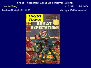
15-251 Classics
Today, we will learn about a formidable tool in probability that will allow us to solve problems that seem really really messy…
Language Of Probability • The formal language of probability is a very important tool in describing and analyzing probability distributions.
Finite Probability Distribution • A (finite) probability distributionD is a finite set S of elements, where each element x in S has a positive real weight, proportion, or probabilityp(x). • The weights must satisfy:
Finite Probability Distribution • A (finite) probability distributionD is a finite set S of elements, where each element x in S has a positive real weight, proportion, or probabilityp(x). • For notational convenience we will define D(x) = p(x). • S is often called the sample spaceand elements x in S are called samples.
Sample space • A (finite) probability distributionD is a finite set S of elements, where each element x in S has a positive real weight, proportion, or probabilityp(x). S Sample space
Probability • A (finite) probability distributionD is a finite set S of elements, where each element x in S has a positive real weight, proportion, or probabilityp(x). S x weight or probability of x D(x) = p(x) = 0.2
Probability Distribution • A (finite) probability distributionD is a finite set S of elements, where each element x in Shas a positive real weight, proportion, or probabilityp(x). S 0.13 0.17 0.1 0.11 0.2 0 0.1 0.06 weights must sum to 1 0.13
Events • A (finite) probability distributionD is a finite set S of elements, where each element x in Shas a positive real weight, proportion, or probabilityp(x). • Any subset E of S is called an event. The probability of event E is
Events • A (finite) probability distributionD is a finite set S of elements, where each element x in Shas a positive real weight, proportion, or probabilityp(x). S Event E
Events • A (finite) probability distributionD is a finite set S of elements, where each element x in Shas a positive real weight, proportion, or probabilityp(x). S 0.17 0 0.1 PrD[E] = 0.4 0.13
Uniform Distribution • A (finite) probability distributionD is a finite set S of elements, where each element x in Shas a positive real weight, proportion, or probabilityp(x). • If each element has equal probability, the distribution is said to be uniform.
proportion of A B to B W B A More Language Of Probability: Conditioning The probability of event A given event Bis written Pr[ A | B ] and is defined to be =
Suppose we roll a white die and black die. What is the probability that the white is 1 given that the total is 7? event A = {white die = 1} event B = {total = 7}
event A = {white die = 1} |A \ B| = Pr[A | B] = Pr[A \ B] = 1/36 |B| Pr[B] 1/6 event B = {total = 7} Can do this because is uniformly distributed. This way does not care about the distribution. • Sample space S = • { (1,1), (1,2), (1,3), (1,4), (1,5), (1,6), • (2,1), (2,2), (2,3), (2,4), (2,5), (2,6), • (3,1), (3,2), (3,3), (3,4), (3,5), (3,6), • (4,1), (4,2), (4,3), (4,4), (4,5), (4,6), • (5,1), (5,2), (5,3), (5,4), (5,5), (5,6), • (6,1), (6,2), (6,3), (6,4), (6,5), (6,6) } Pr[A | B]
1 365/366 364/366 363/366 Another way to calculate Birthday probability Pr(no collision) Pr(1st person doesn’t collide) = 1. Pr(2nd doesn’t | no collisions yet) = 365/366. Pr(3rd doesn’t | no collisions yet) = 364/366. Pr(4th doesn’t | no collisions yet) = 363/366. … Pr(23rd doesn’t| no collisions yet) = 344/366.
A B Independence! • A and B are independent events if • Pr[ A | B ] = Pr[ A ] • • Pr[ A \ B ] = Pr[ A ] Pr[ B ] • • Pr[ B | A ] = Pr[ B ] What about Pr[ A | not(B) ] ?
Independence! • A1, A2, …, Ak are independent events if knowing if some of them occurred does not change the probability of any of the others occurring. E.g., {A_1, A_2, A_3} are independent events if: Pr[A1 | A2 A3] = Pr[A1] Pr[A2 | A1 A3] = Pr[A2] Pr[A3 | A1 A2] = Pr[A3] Pr[A1 | A2 ] = Pr[A1] Pr[A1 | A3 ] = Pr[A1] Pr[A2 | A1 ] = Pr[A2] Pr[A2 | A3] = Pr[A2] Pr[A3 | A1 ] = Pr[A3] Pr[A3 | A2] = Pr[A3]
Independence! • A1, A2, …, Ak are independent events if knowing if some of them occurred does not change the probability of any of the others occurring. Pr[A|X] = Pr[A] for all A = some Ai for all X = a conjunction of any of the others (e.g., A2 and A6 and A7)
Silver and Gold One bag has two silver coins, another has two gold coins, and the third has one of each. One of the three bags is selected at random. Then one coin is selected at random from the two in the bag. It turns out to begold. What is the probability that the other coin is gold?
Let G1 be the event that the first coin is gold. Pr[G1] = 1/2 Let G2 be the event that the second coin is gold. Pr[G2 | G1 ] = Pr[G1 and G2] / Pr[G1] = (1/3) / (1/2) = 2/3 Note: G1 and G2 are not independent.
Monty Hall problem • Announcer hides prize behind one of 3 doors at random. • You select some door. • Announcer opens one of others with no prize. • You can decide to keep or switch. What to do?
Monty Hall problem • Sample space W = • { prize behind door 1, prize behind door 2, prize behind door 3 }. • Each has probability 1/3. Staying we win if we choose the correct door Pr[ choosing correct door ] = 1/3. Switching we win if we choose the incorrect door Pr[ choosing incorrect door ] = 2/3.
why was this tricky? • We are inclined to think: • “After one door is opened, others are equally likely…” • But his action is not independent of yours!
Now, about that formidable tool that will allow us to solve problems that seem really really messy…
If I randomly put 100 letters into 100 addressed envelopes, on average how many letters will end up in their correct envelopes? Hmm… åk k¢Pr(exactly k letters end up incorrect envelopes) = åk k¢ (…aargh!!…)
On average, in class of size m, how many pairs of people will have the same birthday? åk k¢ Pr(exactly k collisions) = åk k¢ (…aargh!!!!…)
HMU • The new tool is called • “Linearity of • Expectation” Expectatus Linearitus
Random Variable • To use this new tool, we will also need to understand the concept of a Random Variable • Today’s lecture: not too much material, but need to understand it well.
Probability Distribution • A (finite) probability distributionD • a finite set S of elements (samples) • each x2S has weight or probabilityp(x)2 [0,1] S 0.05 0.05 0 0.1 0.3 0.2 0.3 weights must sum to 1 “Sample space”
Flip penny and nickel (unbiased) S HH ¼ TT ¼ TH ¼ HT ¼
Flip penny and nickel (biased) heads probability = p S HH p2 TT (1-p)2 TH p(1-p) HT p(1-p)
Probability Distribution S 0.05 0.05 0 0.1 0.3 0.2 0.3
An event is a subset S A 0.05 0.05 0 0.1 0.3 0.2 0.3 Pr[A] = x 2 A p(x) = 0.55
Running Example • I throw a white die and a black die. • Sample space S = • { (1,1), (1,2), (1,3), (1,4), (1,5), (1,6), • (2,1), (2,2), (2,3), (2,4), (2,5), (2,6), • (3,1), (3,2), (3,3), (3,4), (3,5), (3,6), • (4,1), (4,2), (4,3), (4,4), (4,5), (4,6), • (5,1), (5,2), (5,3), (5,4), (5,5), (5,6), • (6,1), (6,2), (6,3), (6,4), (6,5), (6,6) } Pr(x) = 1/36 8 x 2 S E = event that sum ≤ 3 Pr[E] = |E|/|S| = proportion of E in S = 3/36
Random Variable: A measurement for an experimental outcome • Random Variable: a (real-valued) function on S • Examples: • X = value of white die. • X(3,4) = 3, X(1,6) = 1 etc. • Y = sum of values of the two dice. • Y(3,4) = 7, Y(1,6) = 7 etc. • W = (value of white die)value of black die • W(3,4) = 34 Y(1,6) = 16 • Z = (1 if two dice are equal, 0 otherwise) • Z(4,4) = 1, Z(1,6) = 0 etc. • Toss a white die and a black die. • Sample space S = • { (1,1), (1,2), (1,3), (1,4), (1,5), (1,6), • (2,1), (2,2), (2,3), (2,4), (2,5), (2,6), • (3,1), (3,2), (3,3), (3,4), (3,5), (3,6), • (4,1), (4,2), (4,3), (4,4), (4,5), (4,6), • (5,1), (5,2), (5,3), (5,4), (5,5), (5,6), • (6,1), (6,2), (6,3), (6,4), (6,5), (6,6) }
E.g., tossing a fair coin n times • S = all sequences of {H, T}n • D = uniform distribution on S • D(x) = (½)n for all x 2 S • Random Variables (say n = 10) • X = # of heads • X(HHHTTHTHTT) = 5 • Y = (1 if #heads = #tails, 0 otherwise) • Y(HHHTTHTHTT) = 1, Y(THHHHTTTTT) = 0
Notational conventions • Use letters like A, B, E for events. • Use letters like X, Y, f, g for R.V.’s. • R.V. = random variable
Two views of random variables • Think of a R.V. as • a function from S to the reals • or think of the induced distribution on
S HH 2 ¼ TT ¼ 0 TH ¼ 1 HT ¼ Two coins tossed • X: {TT, TH, HT, HH} -> {0, 1, 2} counts the number of heads
Two views of random variables • Think of a R.V. as • a function from S to the reals • or think of the induced distribution on
S HH 2 ¼ TT ¼ 0 TH ¼ 1 HT ¼ Two coins tossed • X: {TT, TH, HT, HH} -> {0, 1, 2} counts the number of heads Distribution on the reals ¼ ¼ ½
Two views of random variables • Think of a R.V. as • a function from S to the reals • or think of the induced distribution on reals
Two dice • I throw a white die and a black die. • Sample space S = • { (1,1), (1,2), (1,3), (1,4), (1,5), (1,6), • (2,1), (2,2), (2,3), (2,4), (2,5), (2,6), • (3,1), (3,2), (3,3), (3,4), (3,5), (3,6), • (4,1), (4,2), (4,3), (4,4), (4,5), (4,6), • (5,1), (5,2), (5,3), (5,4), (5,5), (5,6), • (6,1), (6,2), (6,3), (6,4), (6,5), (6,6) } X = sum of both dice function with X(1,1) = 2, X(1,2)=X(2,1)=3, …, X(6,6)=12
It’s a floor wax and a dessert topping It’s a function on the sample space S. It’s a variable with a probability distribution on its values. You should be comfortable with both views.
From Random Variables to Events • For any random variable X and value a, we can define the eventA that X=a. • Pr(A) = Pr(X=a) = Pr({x 2 S| X(x)=a}).
S HH ¼ TT ¼ TH ¼ HT ¼ Two coins tossed • X: {TT, TH, HT, HH} -> {0, 1, 2} counts the number of heads Pr(X = a) = Pr({x S| X(x) = a}) Pr(X = 1) = Pr({x 2 S| X(x) = 1}) = Pr({TH, HT}) = ½. X 2 ¼ 0 ¼ 1 ½ Distribution on X
Two dice • I throw a white die and a black die. X = sum • Sample space S = • { (1,1), (1,2), (1,3), (1,4), (1,5), (1,6), • (2,1), (2,2), (2,3), (2,4), (2,5), (2,6), • (3,1), (3,2), (3,3), (3,4), (3,5), (3,6), • (4,1), (4,2), (4,3), (4,4), (4,5), (4,6), • (5,1), (5,2), (5,3), (5,4), (5,5), (5,6), • (6,1), (6,2), (6,3), (6,4), (6,5), (6,6) } • Pr(X = 6) • = Pr( {x S : X(x) = 6} ) • = 5/36. Pr(X = a) = Pr({x S: X(x) = a})
From Random Variables to Events • For any random variable X and value a, we can define the eventA that X=a. • Pr(A) = Pr(X=a) = Pr({x 2 S: X(x)=a}). X has a distribution on its values X is a function on the sample space S
