Scheduling
570 likes | 585 Views
Scheduling. Ren-Song Ko National Chung Cheng University. Lecture objectives. To introduce CPU scheduling ’ s role in multiprogrammed operating systems. To describe various CPU-scheduling algorithms. To discuss evaluation criteria for a CPU-scheduling algorithm. Lecture overview.

Scheduling
E N D
Presentation Transcript
Scheduling Ren-Song Ko National Chung Cheng University
Lecture objectives • To introduce CPU scheduling’s role in multiprogrammed operating systems. • To describe various CPU-scheduling algorithms. • To discuss evaluation criteria for a CPU-scheduling algorithm.
Lecture overview • Introduction • Scheduling criteria • Scheduling algorithms • Multiple-processor scheduling • Algorithm evaluation
Introduction • CPU is a one-time investment. • A reasonable thought is to utilize it thoroughly and accomplish as much work as possible. • A common process execution includes an alternating sequence of CPU and I/O activities. • When a process is waiting for I/O results, the CPU then just sits idle. • All this waiting time is wasted; no useful work is accomplished.
A common process execution scenario load Add Write to file cpu burst Wait for I/O I/O burst sub increment read from file cpu burst Wait for I/O I/O burst sub read from file cpu burst Wait for I/O I/O burst
To increase CPU utilization • An intuitive approach to increase CPU utilization is to pick up some useful work when the current running process is waiting for I/O. • That is, CPU could execute another process – multiprogramming. • Thus, OS needs to find a process, if any, for CPU.
Scheduling • But which process? • For example, when P1 is waiting for I/O, we want to find a process, says P2, which only needs CPU for the time less than P1’s I/O. • Hence, P2 execution will not interrupt P1’s execution. • Ideally, P2’s CPU time should equal to P1’s I/O time. • CPU utilization is maximized.
A simple scenario for a good scheduling • CPU utilization 100% • P1: no delay P1 P2 P3 P4 cpu cpu 5 cpu cpu 10 10 15 I/O 30 cpu
Scheduling, cont. • A good scheduling should try to achieve, but not limited to, the following goals: • To minimize the interruption of each process execution • To maximize CPU utilization • However, the goals usually conflict with each other. • The goal should be prioritized depending on the characteristics of computer systems. • Thus, there is no best, only appropriate, scheduling, and scheduling design is critical to system performance.
Scheduler and scheduling algorithm • Whenever the CPU becomes idle, OS must select an appropriate process to be executed. • The part of the operating system that makes this decision is called the scheduler. • The algorithm it uses to make a decision is called the scheduling algorithm.
Nonpreemptive scheduling • OS will invoke the scheduler when a process: • Switches from running to waiting state • Terminates • The scheduling only happening in the above cases is nonpreemptive. • Once the CPU has been assigned to a process, the process keeps the CPU until it releases the CPU either by terminating or by switching to the waiting state. • Can be used on every platform, because it does not require the special hardware such as timer. • Examples are Microsoft Windows 3.x and the Macintosh OS previous to Mac OS X.
Preemptive scheduling • Some OS may also invoke the scheduler when a process: • Switches from running to ready state • Switches from waiting to ready • Such scheduling is preemptive. • Difficult to implement • Consider two processes sharing data. While one is updating the data, it is preempted and then the second one tries to read the inconsistent data. • During the processing of a system call, the kernel may be busy at changing kernel data. What happens if the process is preempted in the middle of these changes? • Examples are Windows 95 and all subsequent versions, and Mac OS X.
Few words about nonpreemptive and preemptive scheduling • As we have seen, preemptive scheduling can suspend a process at an arbitrary instant, without warning. • This leads to race conditions and necessitates semaphores, monitors, messages, or some other sophisticated method for preventing them. • Nonpreemptive scheduling let a process run as long as it wanted to would mean that some process computing π to a billion places could deny service to all other processes indefinitely. • Although nonpreemptive scheduling is simple and easy to implement, it is usually not suitable for general-purpose systems with multiple competing users. • For a dedicated data base server, it may be reasonable for the master process to start a child process working on a request and let it run until it completes or blocks. • The difference is that all processes are under the control of a single master, which knows what each child is going to do and about how long it will take.
What is the next process? • Back in the old days of batch systems, the scheduling algorithm was simple: • Just run the next job • With timesharing systems, the scheduling algorithm is more complex. • There are often multiple users and one or more batch streams. • Even on PCs, there may be several user-initiated processes competing for the CPU, such as networking or multimedia. • Before looking at specific scheduling algorithms, we should think about what the scheduler is trying to achieve. • After all, the scheduler is concerned with deciding on policy, not providing a mechanism. • There are various criteria constituting a good scheduling algorithm.
Scheduling criteria • Some of the possibilities include: • CPU utilization– keep the CPU as busy as possible • Throughput– # of processes that complete their execution per time unit • Turnaround time– the interval from the time of submission of a process to the time of completion • Waiting time– amount of time a process has been waiting in the ready queue • Response time– amount of time it takes from when a request was submitted until the first response is produced, not output (for interactive environment) • Fairness– make sure each process gets its fair share of the CPU
Optimization problems • Most of criteria a scheduler is trying to achieve can be easily defined as an optimization problem. • Maximize CPU utilization • Maximize throughput • Minimize turnaround time • Minimize waiting time • Minimize response time
Scheduling criteria • A little thought will show that some of these goals are contradictory. • To minimize response time for interactive users, the scheduler should not run any batch jobs at all. • However, it violates turnaround time criterion for the batch users. • It can be shown (Kleinrock, 1975) that any scheduling algorithm that favors some class of jobs hurts another class of jobs. • The amount of CPU time available is finite, after all. • To give one user more you have to give another user less.
Scheduling algorithms • First-Come, First-Served (FCFS) • Round-Robin (RR) • Priority scheduling • Multilevel Feedback-Queues • Shortest-Job-First (SJF) • Time-Sharing • Time-Slice • Lottery scheduling
First-Come, First-Served (FCFS) • CPU is allocated to the process that requests the CPU first. • Can be easily managed with a FIFO queue. • When a process enters the ready queue, it is linked onto the tail of the queue. • When the CPU is free, the process at the head of the queue will be assigned to the CPU and then removed from the queue. • The average waiting time, however, is often quite long. • Specially, there is a long process in front of short processes.
P1 P2 P3 0 18 24 30 FCFS example ProcessBurst Time P1 18 P2 6 P3 6 • Suppose that the processes arrive in the order: P1 , P2 , P3 The Gantt Chart for the schedule is: • Waiting time for P1 = 0; P2 = 24; P3 = 27 • Average waiting time: (0 + 24 + 27)/3 = 17
Waiting time • (competition – arrival) – CPU P1 : (18 – 0) – 18 = 0 P2 : (24 – 0) – 6 = 18 P3 : (30 – 0 ) – 6 = 24 Average Waiting Time = (0+18+24)/3 = 14
Round-Robin (RR) • Each process is assigned a time interval, quantum, which it is allowed to run. • If the process is still running at the end of the quantum, the CPU is preempted and given to another process. • If the process has blocked or finished before the quantum has elapsed, the CPU switching is done when the process blocks, of course. • Round robin is easy to implement via queue. • When the process uses up its quantum, it is put on the end of the queue.
P1 P2 P3 P4 P1 P2 P3 P4 P1 P4 0 10 20 30 40 50 55 65 75 80 90 RR example, quantum = 10 ProcessBurst Time P1 25 P2 15 P3 20 P4 30 • The Gantt chart is: • Typically, higher average turnaround than SJF, but better response
RR Performance • If there are n processes in the ready queue and the time quantum is q, then each process gets 1/n of the CPU time in chunks of at most q time units at once. No process waits more than (n-1)q time units. • What is the length of the quantum? • Switching from one process to another, called context switch, requires a certain amount of time for doing the administration, says 5 ms. • E.g., saving and loading registers and memory maps, updating various tables and lists, etc. • Suppose that this process switch or context switch, • Suppose that the quantum is set at 20 ms. • After doing 20 ms of useful work, the CPU will have to spend 5 ms on process switching. • 20% of the CPU time will be wasted on administrative overhead.
RR Performance, cont. • To improve the CPU efficiency, set the quantum to 500 ms. • Now the wasted time is less than 1%. • But consider there are ten processes and the first one gets the chance to run. • The second one may not start until about 1/2 sec later, and so on. • The unlucky last one may have to wait 5 sec. • Most users will perceive a 5-sec response to a short command as terrible. • The conclusion can be formulated as follows: • setting the quantum too short causes too many process switches and lowers the CPU efficiency • setting it too long may cause poor response to short interactive requests, i.e., FCFS. • A quantum around 100 ms is often a reasonable compromise.
Time Quantum and Context Switch Time 20 15 10 15 10 1 14 15
Priority scheduling • RR implicitly assumes that all processes are equally important. • Frequently, some are more important than others. • For example, a daemon process sending email in the background should be assigned a lower priority than a process displaying a video film on the screen in real time. • A priority number (integer) is associated with each process • The CPU is allocated to the process with the highest priority (smallest integer ←→ highest priority) • preemptive • nonpreemptive • Problem: starvation → low priority processes may never execute • Solution: aging → decrease the priority of the currently running process at each clock tick
P3 P4 P1 P2 P4 32 36 38 0 12 2 Nonpreemptive priority scheduling example Process Burst TimePriority P1 4 4 P2 10 2 P3 2 1 P4 20 3 P5 2 5 • The Gantt chart for the schedule is: • Average waiting time = (6 + 0 + 16 + 18 + 1)/5 = 8.2
Preemptive priority scheduling example Process Burst TimePriorityArrival Time P1 4 4 0 P2 10 2 2 P3 2 1 4 P4 20 3 6 P5 2 5 8 • The Gantt chart for the schedule is: P1 P5 P2 P3 P2 P4 P1 4 6 14 34 36 38 0 2
Priority scheduling, cont. • It is often convenient to group processes into priority classes managed by different queues. • Priority scheduling is used among queues. • Each queue may has its own scheduling algorithm. • Consider a system with five priority queues. The scheduling algorithm is as follows: • As long as there are processes in priority 5, just run each one in round-robin fashion, and never bother with lower priority processes. • If priority 5 is empty, then run the priority 4 processes round robin. • If priorities 5 and 4 are both empty, then run priority 3 round robin. and so on. • Note that priority scheduling among queues may cause lower priority processes starve to death. • A solution to avoid starvation is to use Time-Slice scheduling among queues. • For example, each queue gets a certain amount of CPU time which it can schedule amongst its processes; e.g., they may have 50%, 20%, 15%, 10%, and 5% of CPU time respectively.
Multilevel Feedback-Queues • One of the earliest priority schedulers was in CTSS, 1962. • CTSS had the problem that process switching was very slow because the 7094 could hold only one process in memory. • Each switch meant swapping the current process to disk and reading in a new one from disk. • It was more efficient to give CPU-bound processes a large quantum once, rather than giving them small quanta frequently (to reduce swapping). • However, giving processes a large quantum means poor response time. • The solution is to give higher priority processes less quanta and low priority processes more quanta. • Whenever a process used up the quanta, its priority was decreased. • As the process sank deeper into the priority queues, it would be run less frequently, saving the CPU for short interactive processes. • If a process waits too long in a low priority queue, it may be moved to a higher priority queue. • This prevents starvation.
Multilevel Feedback-Queues example • Three queues: • Q0– RR with time quantum 8 milliseconds • Q1– RR time quantum 16 milliseconds when Q0 is empty • Q2– FCFS but only Q0 and Q1 are empty • Scheduling • A new job enters queue Q0. When it gains CPU, job receives 8 milliseconds. If it does not finish in 8 milliseconds, job is moved to queue Q1. • At Q1 job receives 16 additional milliseconds. If it still does not complete, it is preempted and moved to queue Q2.
Multilevel Feedback-Queues example, cont. p1: Time: 30 p1: Time: 22 p1: Time:6
Shortest-Job-First (SJF) • Simply a priority algorithm where the priority is the inverse of the (predicted) run time. • The larger the run time, the lower the priority, and vice versa. • Appropriate for batch jobs for which the run times are known in advance. • Two schemes: • nonpreemptive • Preemptive, Shortest-Remaining-Time-First (SRTF) • if a new process arrives with run time less than remaining time of executing process, preempt • SJF is optimal – gives minimum average waiting time
Nonpreemptive SJF example Process Arrival TimeBurst Time P1 0.0 8 P2 2.0 5 P3 3.0 3 P4 5.0 5 • SJF (non-preemptive) • Average waiting time = (0 + 6 + 3 + 7)/4 = 4 P1 P3 P2 P4 8 11 16 21 0
Preemptive SJF example Process Arrival TimeBurst Time P1 0.0 8 P2 2.0 5 P3 3.0 3 P4 5.0 5 • SJF (preemptive) • Average waiting time = (9 + 1 + 0 +2)/4 = 3 P1 P2 P3 P2 P4 P1 2 3 6 10 15 21 0
Run time estimation • SJF is optimal, the only problem is figuring out which process is the shortest one. • Note that SJF is only optimal when all processes are available simultaneously. • Counter example • Five processes, Athrough E, with run times of 2, 4, 1, 1, and 1, respectively. • Arrival times are 0, 0, 3, 3, and 3. • SJF will pick the processes in the order A,B,C,D,Efor an average wait of 4.6. • However, running them in the order B,C,D,E,Ahas an average wait of 4.4. • One approach is to make estimates based on past behavior.
Exponential averaging 1. tn = actual length of nth cpu burst 2. n+1 = predictive value for the next cpu burst 3. , 0≤≤1 4. Define : n+1 = tn+(1 - ) n
Exponential averaging, cont. • =0 • n+1 = n • Recent history does not count • =1 • n+1 = tn • Only the actual last run time counts • If we expand the formula, we get: n+1 = tn+(1 - ) tn-1+ … +(1 - )j tn-j+ … +(1 - )n +1 0 • Since both and (1 - ) are less than or equal to 1, each successive term has less weight than its predecessor
Time-Sharing • Prioritized credit-based – process with most credits is scheduled next • Crediting based on factors including priority and history • Credit subtracted when timer interrupt occurs • When credit = 0, another process chosen • When all processes have credit = 0, recrediting occurs • One example is Linux
Time-Sharing example • The kernel maintains a list of all processes in a multiple queues structure. • Each queue contains two priority arrays - active and expired. • The active array contains all tasks with time remaining in their time slices. • The expired array contains all expired tasks. • The scheduler chooses the process with the highest priority from the active array. • When the process have exhausted its time slices, it will be moved to the expired array. • When the active array is empty, the two arrays are exchanged. • The expired array becomes the active array, and vice versa.
Time-Slice • Consider a system with n processes, all things being equal, each one should get 1/n of the CPU cycles. • The system keeps track of how much CPU each process has had since its creation. • Compute the amount of CPU each one is entitled to. • Compute the ratio of actual CPU had to CPU time entitled. • A ratio of 0.5 means that a process has only had half of what it should have had. • A ratio of 2.0 means that a process has had twice as much as it was entitled to. • The algorithm is then to run the process with the lowest ratio until it is not the lowest. • It can be easily modified so that each process gets a certain amount of CPU time based on priority.
Lottery scheduling • Time-Slice is difficult to implement. • Lottery scheduling give similarly predictable results with a much simpler implementation. • The basic idea is to give processes lottery tickets for CPU time. • Whenever a scheduling decision has to be made, a lottery ticket is chosen at random, and the process holding that ticket gets the CPU. • E.g., the system might hold a lottery 50 times a second, with each winner getting 20 ms of CPU time as a prize. • More important processes can be given extra tickets, to increase their odds of winning. • If there are 100 tickets outstanding, and one process holds 20 of them, it will have a 20 percent chance of winning each lottery, which is about 20 percent of the CPU.
Lottery scheduling • In contrast to a priority scheduler, where it is very hard to state what having a priority of 40 actually means. Here the rule is clear: • a process holding a fraction f of the tickets will get about a fraction f of the CPU time. • Lottery scheduling can be used to solve problems that are difficult to handle with other methods. • One example is a video server in which several processes are feeding video streams to their clients, but at different frame rates. • Suppose that the processes need frames at 10, 20, and 25 frames/sec. • By allocating these processes 10, 20, and 25 tickets, respectively, they will automatically divide the CPU in the correct proportion.
Policy versus mechanism • So far, we assumed that all the processes belong to different users and are thus competing for the CPU. • However, sometimes a process has many children under its control. • A server process may have many children working on different requests. • The main process know which of its children are the most important. • Without any input from user processes, the scheduler rarely makes the best choice. • The solution is to separate the scheduling mechanism from the scheduling policy. • The scheduling algorithm is parameterized in some way, and the parameters can be filled in by user processes. • Suppose that the kernel uses a priority scheduling algorithm but provides a system call by which a process can set the priorities of its children. • In this way the parent can control in detail how its children are scheduled, even though it itself does not do the scheduling. • Here the mechanism is in the kernel but the policy is set by a user process.
Multiple-processor scheduling • Load sharing becomes possible if multiple CPUs are available. • The scheduling problem becomes more complex, and there is no one best solution. • Consider systems in which the CPUs are identical, or homogeneous, in terms of their functionality; • Any CPU can run any process in the queue. • Two approaches • Asymmetric multiprocessing– a single CPU makes all scheduling decisions; the others execute only process • only one CPU accesses the system data structures, no need for data sharing • Symmetric multiprocessing (SMP)– each CPU is self-scheduling • The scheduler for each CPU select a process to execute • Need to ensure that two CPUs do not choose the same process and that processes are not lost from queue
Processor affinity versus load balancing • Processor affinity • A process has an affinity for the CPU on which it is currently running • To avoid migration of processes because of the high cost of invalidating and repopulating caches • Load balancing • To keep the workload evenly distributed across all CPUs • Push migration • A specific task periodically checks the load on each CPU and evenly distributes the load if an imbalance is found • Pull migration • An idle CPU pulls a waiting task from a busy CPU • Load balancing often counteracts the benefits of processor affinity • No absolute rule concerning what policy is best