
1. Interpolating polynomials
E N D
Presentation Transcript
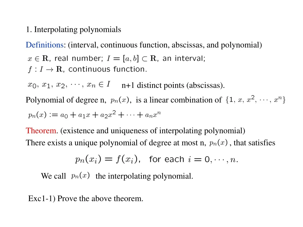
1. Interpolating polynomials Definitions: (interval, continuous function, abscissas, and polynomial) Polynomial of degree n, , is a linear combination of n+1 distinct points (abscissas). Theorem. (existence and uniqueness of interpolating polynomial) There exists a unique polynomial of degree at most n, , that satisfies We call the interpolating polynomial. Exc1-1) Prove the above theorem.
Lagrange form of interpolating polynomial. (Has a simple form and useful for the error estimation.) Derive an interpolating polynomial for points, Defining the Lagrange polynomial by Lagrange form of interpolating polynomial is written Theorem: (Interpolation Error) If a function f is continuous on [a,b] and has n+1 continuous derivatives on (a,b), then for 8 x2[a,b], 9 x(x)2(a,b), such that
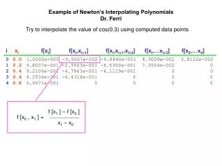
Newton form of interpolating polynomial. We construct an interpolating polynomial for f(x) in the above form, that is, satisfies Definition (Divided difference) The zeroth divided difference w.r.t. the point is written The kth divided difference of f w.r.t. the points is
Newton form of interpolating polynomial is written namely, Newton form is more efficient; fewer operation to determine its coefficients. Particularly, when a new data points become available, Newton form allows them to be incorporated easily. • Interpolation error in Newton form can be derived as follows:
Exc 1-2) Derive the Newton form of interpolating polynomial, Exc 1-3) Show, for any permutation Exc 1-4) Check that the interpolating error formula in Newton form is identical to hint: apply the generalized Rolle’s theorem to to show
Runge’s phenomenon. When approximating the function f(x) on [a,b] by an interpolating polynomial, an error does not necessary decrease as increase the degree of polynomial. The interpolation oscillates to the end of the interval, Limitation of the interpolating polynomials Also consider a function which is singular at x = 0. cf) Gibbs phenomenon When approximating a periodic piecewise differentiable function f(x) by the Fourier series, an error near to the discontinuity of f(x) does not decrease as increasing the number of Fourier series.
Theorem: (Weierstrass) Idea of a proof) A following polynomial has this property. The Bernstein polynomials {bn,i} converges uniformly to f(x) on [0,1] Theorem: (Faber) There is no universal node matrix (which is a sequence of abscissas with increasing points), for which the corresponding interpolation polynomials converges to 8 f(x)2C[a,b] . Some more theorems.
(1) Use optimal points for abscissas for the interpolation: Chebyshev points (roots of Chebyshev polynomial) minimize Roots of Legendre polynomial minimize Use piecewise polynomial interpolation with lower degree, such as Piecewise linear interpolation, Spline interpolation, Hermite interpolation. ex) Cubic Hermite: Interpolation How to overcome the problem.
Exc1-5) Programing: a). Make a code for the interpolation polynomial in Lagrange form and Newton form. (It is allowed to use a code from the lecture.) b). Compare execution time. Check if your procedure is optimal. c). Using Chebyshev points, estimate errors in for different degrees of interpolating polynomial n such as n = 2n , n =2 to 7 d). (optional) Using the roots of Legendre polynomial, redo c). Exc1-6) Numerically confirm that the interpolating polynomial based on the Bernstein polynomial converges to the Runge’s function on [-1,1]. (Note: the Bernstein polynomials in this note is defined on [0,1].)