Download
1 / 31
310 likes | 411 Views
Explore the SDSS galaxy samples, analyze BAO in SDSS DR7 Main Galaxy Sample, study correlation functions, and project 3D data into 2D slices for further insights into galaxy clustering and cosmology. Utilize tomography techniques to enhance understanding of redshift space distortions and spatial correlations in large-scale structures. Discover significant features in the correlation functions for galaxies in SDSS data and Millennium simulations. Implement advanced computations on GPUs for efficient data processing and analysis in SDSS database. Enhance the detection of BAO features and cosmological signatures in galaxy distributions through innovative tomographic methods and correlation analyses.

E N D
BAO and Tomography of the SDSS Alex SzalayHaijun TianTamas BudavariMark Neyrinck
SDSS Redshift Samples • Main Galaxies • 800K galaxies, high sampling density, but not too deep • Volume is about 0.12 Gpc3 • Luminous Red Galaxies • 100K galaxies, color and flux selected • mr < 19.5, 0.15 < z < 0.45, close to volume-limited • Quasars • 20K QSOs, cover huge volume, but too sparse
Finding the Bumps – DR4 • Eisenstein et al (2005) – LRG sample
Primordial Sound Waves in SDSS Power Spectrum (Percival et al 2006, 2007) SDSS DR6+2dF SDSS DR5 800K galaxies
(r) from linear theory + BAO • Mixing of 0 , 2 and 4 • Along the line of sight r
2D Symmetry • There is a planar symmetry: • Observer+ 2 galaxies • Thus 2D correlation of a slice is the same • We usually average over cos • Very little weight along the axis: • Sharp of features go away
Tomography of SDSS • SDSS DR7 Main Galaxy Sample • Limit distances to 100<r<750 h-1Mpc • Cut 3D data into thin angular slices • Project down to plane (only 2D info) • Different widths (2.5, 5, 10 deg) • Rotate slicing direction by 15 degrees • Analyze 2D correlation function (,) • Average over angle for 1-D correlations
Why correlation function? • For a homogeneous isotropic process,the correlation function in a lower dimsubset is identical • There are subtleties: • With redshift space distortions the process is not fully homogeneous and isotropic • Redshift space distortions and ‘bumps’ • Distortions already increase the ‘bumps’ • Any effects from the ‘slicing’?
Projection and Slicing Theorem The basis of CAT-SCAN / Radon xform
Slices of finite thickness • Project redshift-space power spectrum with a corresponding window functionsinc(kzR) • Anisotropic power spectrum • There is a thickness-dependent effect • Thinner slices give bigger boost
(r) along the line of sight Average of all 2.5 degree slices
(r) along the line of sight • The correlation function along a 1D line: • Pencilbeam • Corresponding power spectrum • Projection of P(s)(k) onto a single axis
Computations on GPUs • Generated 16M randoms with correctradial and angular selection for SDSS-N • Done on an NVIDIA GeForce 260 card • 400 trillion galaxy/random pairs • Brute force massively parallel code muchfaster than tree-code • All done inside the JHU SDSS database • 2D correlation function is now DB utility
Summary • Redshift space distortions amplify features • Lower dimensional subsets provide further amplification of ‘bumps’ at 107-110h-1Mpc • Boost much stronger along the line of sight • Using these techniques we have strong detection of BAO in SDSS DR7 MGS • Effect previously mostly seen in LRGs • Trough at 55h-1Mpc is a harmonic, sharpness indicates effects of nonlinear infall • Bump at 165h-1Mpc puzzling
Cosmology used M = 0.279 L = 0.721 K = 0.0 h= 0.701 w0 = -1