Regional Air Pollution Study
320 likes | 407 Views
This study evaluates the spatial representativeness of air quality monitors in the WRAP region using data from the IMPROVE Network. It aims to provide insights into regional air pollution patterns for better environmental management. The study includes methodology, analysis, and results for various physiographic regions.

Regional Air Pollution Study
E N D
Presentation Transcript
Regional Air Pollution Study Alissa Dickerson, M.S. Environmental Specialist Enviroscientists, Inc.
Goal of Study • Western Regional Air Partnership (WRAP) http://wrapair.org • Causes of Haze Assessment (COHA) • Goal: provide assessment of Class I areas through integrated approach • www.coha.dri.edu
Overview • Introduction • Methodology • Analysis • Results & Discussion: Case Studies • Summary
What is Spatial Representativeness? • Area within which pollutant concentrations are approximately constant • Quantitative and qualitative approach to investigate equivalency of measurements
Why is it important? • Data assessments can determine dependence and elicit solutions • Comprehensive picture of a complex system • Tool to assess degree to which measured concentrations can be derived from reference points • Optimal network design
Why is it Important? (cont.) • Evaluation tool to help more efficiently in mediation of environmental problems • Understanding regional visibility & reduction
Introduction • Visibility reduction 1977 CAA • USEPA Regional Haze Rule, Final (40 CFR 51, 1999) • Interagency Monitoring of Protected Visual Environments = IMPROVE (1985) • 5 regional organizations
The IMPROVE Network: Objectives • Federally mandated Class I areas • National parks, monuments, wilderness areas • Identify current conditions of visibility • Determine aerosol species and sources • Document trends • Cultivate representative monitoring network
The IMPROVE Network • 163 sites • 1-in-3 day sampling • 4 cyclone-based modules • Coarse mass & speciated fine aerosols
The Improve Network bext visibility • Light Extinction Formula • bext= 3*f(RH)[Sulfate] + 3*f(RH)[Nitrate] + 4*[Organic Carbon] + 10*[Elemental Carbon] + 1*[ Fine Soil] + 0.6*[Coarse Mass]+ 10 • Concentrations [ ] Units=μg/m3 • Units= Mm-1, proportional to amount of light lost over distance of 1 million meters • Rayleigh Scattering= 10 Mm-1, proportional 0.0 deciviews or 400 km
Research Objectives • Determine spatial representativeness of IMPROVE monitors- WRAP • WA, OR, CA, NV, ID, ND, SD, CO, AZ, NM, TX • 14 Physiographic Regions
Considerations • What are most dominant chemical species during 20% worst visibility days within a region? • What are practical statistical and spatial analysis methods? • How do concentrations vary by season?
Considerations • How can expected average concentrations be determined for a region? • What is a method to test validity?
Methodology • Data • 1997-2002, 54 monitors w/most complete data • Six aerosol species • Sulfates, nitrates, organic carbon (OC), elemental carbon (EC), fine soil, coarse mass (CM) • Focus: Upper 20% of calculated visibility impairment values or 20% worst visibility days
Assumptions • All elemental sulfur is from sulfate -> ammonium sulfate • All nitrate -> ammonium nitrate • Total organic carbon= C released in four steps (OC1-OC4) + pyrolized organics (OP) Thermal Optical Reflectance (TOR) analysis of quartz filter
Assumptions • Elemental carbon (light absorbing carbon) = EC fractions (EC1-EC3) – pyrolized organics (OP) TOR analysis of quartz filter • Fine soil = sum of Al, Si, K, Ca, Ti particle-induced X-ray emission (PIXE) & Fe X-ray fluorescence (XRF) • Coarse mass = total mass - fine mass
Analysis Procedures • 1) Characterize dynamics of regions • Climate & meteorology: wind patterns & back-trajectory analysis (transport) • Graphically displays % of time an air mass spent in an area • Color coded (shading increases w/ residence) • Topography: elevation & intervening terrain • Emission sources and population centers
Analysis Procedures (cont.) • 2) Regional spatial correlation analysis: correlation expected to decrease w/distance • Correlation matrix of aerosol measurements • Distance matrix (km) • Consideration • Correlation of site vs. itself = unity [Artificial]= uncertainty * random #+measurement • [Artificial] plotted at distance of 0
Analysis (cont.) • 3) Criteria correlation cut-off = 0.7 • Rationalize association between monitoring sites • Validation of spatial representativeness • 4) Seasons • Warm months: April to September • Cold months: October to March
Analysis (cont.) • 5) Expected average concentrations • density (like temp.) of atmosphere varies w/ altitude • [Estimated] = [aerosol]* site density density @ sea level • Put conc. into elevation ranges based on natural breaks, then averaged= regional estimated conc. • Uncertainty= standard deviation of average concentrations within elevation range (applicable only with 2 or more sites)
Analysis (cont.) • 6) Test of representativeness • Analyzed sites within each region • Calculated seasonal average concentrations • Uncertainty= average measurement uncertainty • Compared to estimated concentrations
3.The Northern Great Plains Region • Characteristics • (E) Montana, (NE) Wyoming, & (W) portions of North and South Dakota • Terrain: mostly prairie & rolling hills, mix of forest and grassland • Badlands composed of steep buttes and pinnacles • Sparse population centers • Several coal-fired power plants, west-central ND
Residence Time Analysis WICA1 • Warm months • Prevailing winds SE • Bring in dry air from SW U.S. • Moist warm air masses from Gulf of Mexico • Few inversions
Residence Time Analysis MELA1 • Cold months • Cold continental air flowing from N/NW from Canada • L system typical, flushes atmosphere
Test SitesFOPE1 (2yr) NOCH1 (2 yr) FOPE1 30m elev. difference MELA1 [NO3]=0.9 µg/m3
Northern Great Plains Regional Conclusions • Relatively flat terrain with good dispersion of air • Atypical stagnation alleviates regional haze problems during most days • SO4 • representative ~ 180km • Colder months show good agreement out to 700 km
Northern Great Plains Regional Conclusions (cont.) • NO3 • Rep. Distance ~ 450 km, 200km warm months • Factor – chemical nature to volatilize quickly in warmer temperatures or not form at all • OC • Southerly located IMPROVE samplers recorded higher OC concentrations on worst visibility days • Forest fire episodes • Rep. distance (Southern region) ~250 km
Thank you Questions?