Download
1 / 51
510 likes | 677 Views
Acurate determination of parameters for coarse grain model. Simulated systems:. Total 15 simulations using GROMACS of DPPC, POPC, and DOPC bilayers with cholesterol at 0%, 10%, 20%, 25%, and 33% concentrations (total 200 lipids in each system).

E N D
Simulated systems: • Total 15 simulations using GROMACS of DPPC, POPC, and DOPC bilayers with cholesterol at 0%, 10%, 20%, 25%, and 33% concentrations (total 200 lipids in each system). • At 1 atm pressure (semi-isotropic). DPPC mixtures at 323 K and DOPC, POPC mixtures at 303 K. • PME with 1 nm real space cut off. • VDW with 1.8 nm cut off. • Force field parameters developed in our group. (Contact for parameters: pandit@cs.purdue.edu, schiu@ncsa.uiuc.edu) • Simulated for 30 ns. Last 10 ns used in averaging. One DPPC+cholesterol at 1:1 is simulated for 20 ns. Used last 5 ns for volume computation.
Pure systems and comparison with experiments: Experimental data from Prof. John Nagle.
The system is divided into three regions. Water, headgroup (HG) and hydrocarbon core. • Component volumes (vi)are computed by the method proposed by Feller et al.1,where the system is divided into ns slabs and the function is optimized. • The hydrocarbon thickness (Dc) is calculated by Gibbs surface method. • The area per lipid (Al) is Vc/Dc. Pure systems and comparison with experiments: 1Armen, R, Uitto, O, and Feller, S, Biophys. J., 75, 734 (1998)
Pure systems and comparison with experiments: 1 Kucerka, N. et al, Biophys. J., L83, (2006); 2 Kucerka, N. et al, J. Membrane Biol. 208, 193 (2005).
Pure systems and comparison with experiments: • The difference between Al and Alg is approximately 4%, 5%, and 7.5% for DPPC, POPC and DOPC bilayers respectively. • We will consider Al as lipid area instead of Alg because • It is experimentally determined • The Alg depends on the parameters of pressure coupling algorithm and other simulation parameters.
Cholesterol mixtures and comparison with experiments: • Partial molecular volume • Partial molecular area1 1Edholm, O and Nagle, J F, Biophys. J., 89, 1827 (2005)
Cholesterol mixtures and comparison with experiments: Greenwood et. al,Chem. Phys. Lipids, 143, 1 (2006)
Cholesterol mixtures and comparison with experiments: Greenwood et. al,Chem. Phys. Lipids, 143, 1 (2006)
Cholesterol mixtures and comparison with experiments: 1Greenwood et. al,Chem. Phys. Lipids, 143, 1 (2006)
b - side a - side • The cholesterol packs preferentially with the -side toward Sn-1 chain of POPC and -side towards Sn-2 chain.
Our force fields are accurately reproducing structural properties of the bilayers. • Two sides of cholesterol play important role in structual organization in bilayers.
Coarse grain mapping 3D lipid bilayer 2D lattice field lipid chain Lattice field si Cholesterol Hard rod Khelashvili, Pandit and Scott., J. Chem. Phys. (2005), 123, 034910.
where Lipid chains as order parameter field si is the order parameter of a chain. We consider average effect of the neighboring chains (Mean field approximation) Khelashvili, Pandit and Scott., J. Chem. Phys. (2005), 123, 034910.
Lipid chains as order parameter field We write a self-consistent equation as where the conformations of the chains are taken from a MD simulation of 1600 DPPC bilayer at 50 C (appropriately transformed). Tune V0 to get correct phase transition temperature. Khelashvili, Pandit and Scott., J. Chem. Phys. (2005), 123, 034910.
Binary mixture of DPPC and cholesterol • Cholestrols are considered as rigid rods diffusing through the lattice field of the chain order parameters. • The coupling coefficients between DPPC and cholesterol are determined by fitting a straight line to cholesterol-DPPC chain interaction energy vs. si plot. • The cholesterol positions and orientations are updated at the each step using Time dependent Ginzburg-Landau equation (TDGL) and then the lipid order parameters are updated by solving appropriate self-consistent equations. Khelashvili, Pandit and Scott., J. Chem. Phys. (2005), 123, 034910.
Coarse grain dynamics Initialize order parameter field, place cholesterol randomly, and initialize MD chain libraries at given temperature Solve self-consistent equation to equilibrate Order parameter field around cholesterol positions. Move cholesterol rods using TDGL equations Khelashvili, Pandit and Scott., J. Chem. Phys. (2005), 123, 034910.
Binary mixture of DPPC and cholesterol Order parameter fields after 20 s of simulation with 10000 chains and 7%, 11%, 18%, 25% and 33% cholesterols. Khelashvili, Pandit and Scott., J. Chem. Phys. (2005), 123, 034910.
Binary mixture of DPPC and cholesterol Pandit et al., Biophys. J. (2007), 123, 034910.
Binary mixture of DPPC and cholesterol Pandit et al., Biophys. J. (2007), 123, 034910.
Modeling mixture of lipids (on going work) Composition field: Where ’s are the volume fractions of the lipids. Where C is the concentration of SM in the system. i ‘s are evolved using Cahn-Hilliard model
Bond order for C-C bond Bond order interaction • Uncorrected bond order: • Where is for • andbonds • The total uncorrected bond order • is sum of three types of bonds • Bond order requires correction to • account for the correct valency 1 van Duin et al , J. Phys. Chem. A, 105, 9396 (2001)
Bond Order Interaction • After correction, the bond order between a pair of atoms depends on the uncorrected bond orders of the neighbors of each atoms • The uncorrected bond orders are stored in a tree structure for efficient access. • The bond orders rapidly decay to zero as a function of distance so it is reasonable to construct a neighbor list for efficient computation of bond orders
Neighbor Lists for Bond Order • Efficient implementation critical for performance • Implementation based on an oct-tree decomposition of the domain • For each particle, we traverse down to neighboring octs and collect neighboring atoms • Has implications for parallelism (issues identical to parallelizing multipole methods)
Other Local Energy Terms • Other interaction terms common to classical simulations, e.g., bond energy, valence angle and torsion, are appropriately modified and contribute to non-zero bond order pairs of atoms • These terms also become many body interactions as bond order itself depends on the neighbors and neighbor’s neighbors • Due to variable bond structure there are other interaction terms, such as over/under coordination energy, lone pair interaction, 3 and 4 body conjugation, and three body penalty energy
Non Bonded van der Waals Interaction • The van der Waals interactions are modeled using distance corrected Morse potential • Where R(rij)is the shielded distance given by
Electrostatics • Shielded electrostatic interaction is used to account for orbital overlap of electrons at closer distances • Long range electrostatics interactions are handled using the Fast Multipole Method (FMM).
Charge Equilibration (QEq) Method • The fixed partial charge model used in classical simulations is inadequate for reacting systems. • One must compute the partial charges on atoms at each time step using an ab-initio method. • We compute the partial charges on atoms at each time step using a simplified approach call the Qeq method.
Charge Equilibration (QEq) Method • Expand electrostatic energy as a Taylor series in charge around neutral charge. • Identify the term linear in charge as electronegativity of the atom and the quadratic term as electrostatic potential and self energy. • Using these, solve for self-term of partial derivative of electrostatic energy.
Qeq Method We need to minimize: subject to: where
Qeq Method From charge neutrality, we get:
Qeq Method Let where or
Qeq Method • Substituting back, we get: We need to solve 2n equations with kernel H for si and ti.
Qeq Method • Observations: • H is dense. • The diagonal term is Ji • The shielding term is short-range • Long range behavior of the kernel is 1/r Hierarchical methods to the rescue! Multipole-accelerated matrix-vector products combined with GMRES and a preconditioner.
Hierarchical Methods • Matrix-vector product with n x n matrix – O (n2) • Faster matrix-vector product • Matrix-free approach • Appel’s algorithm, Barnes-Hut method • Particle-cluster interactions – O (n lg n) • Fast Multipole method • Cluster-cluster interactions – O (n) • Hierarchical refinement of underlying domain • 2-D – quad-tree, 3-D – oct-tree • Rely on decaying 1/r kernel functions • Compute approximate matrix-vector product at the cost of accuracy
Hierarchical Methods … • Fast Multipole Method (FMM) • Divides the domain recursively into 8 sub-domain • Up-traversal • computes multipole coefficients to give the effects of all the points inside a node at a far-way point • Down-traversal • computes local coefficients to get the effect of all far-away points inside a node • Direct interactions – for near by points • Computation complexity – O ((d+1)4n) • d – multipole degree
Hierarchical Methods … • Hierarchical Multipole Method (HMM) • Augmented Barnes-Hut method or variant of FMM • Up-traversal • Same as FMM • For each particle • Multipole-acceptance-criteria (MAC) - ratio of distance of the particle from the center of the box to the dimension of the box • use MAC to determine if multipole coefficients should be used to get the effect of all far-away points or not • Direct interactions – for near by points • Computation complexity – O ((d+1)2n lg n)
Qeq: Parallel Implementation • Key element is the parallel matrix-vector (multipole) operation • Spatial decomposition using space-filling curves • Domain is generally regular since domains are typically dense • Data addressing handled by function shipping • Preconditioning via truncated kernel • GMRES never got to restart of 10!
Qeq Parallel Performance Size corresponds to number of atoms; all times in seconds, speedups in parentheses. All runtimes on a cluster of Pentium Xeons connected over a Gb Ethernet.
Qeq Parallel Performance Size corresponds to number of atoms; all times in seconds, speedups in parentheses. All runtimes on an IBM P590.
Parallel ReaX Performance • ReaX potentials are near-field. • Primary parallel overhead is in multipole operations. • Excellent performance obtained over rest of the code. • Comprehensive integration and resulting (integrated) speedups being evaluated.