Download

1 / 20
210 likes | 448 Views
2 . 3. Bounding Volumes. Bounding volumes of use for collision detection. Bounding Volumes. Simple implicit/explicit bounding volumes for complex geometry. Introduction to Bounding Volumes.

E N D
2.3.Bounding Volumes Bounding volumes of use for collision detection
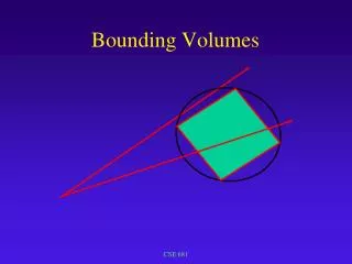
Bounding Volumes Simple implicit/explicit bounding volumes for complex geometry
Introduction to Bounding Volumes A bounding volume is simply a volume that bounds (i.e. encapsulates) one, or more, objects. Bounded objects can have arbitrarily complex geometry. A geometrically simple bounding volume entails that collision tests can be initially against the bound (permitting fast rejection), followed by a more complex and accurate collision test if needed. In some applications, the bounding volume intersection suffices to determine intersection between the bounded objects.
Ideal characteristics of a bounding volume Ideally a bounding volume should: Provide an inexpensive test for intersection Fit tightly around the bounded object(s) Be inexpensive to compute Be easy transformed (e.g. rotated) Require little memory for storage Often, the above characteristics are mutually opposed to one another.
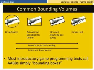
Bounding volume local coordinate systems Bounding volumes are typically specified in object (or model) space. In order to test for collision, the bounding volumes need to be expressed within a common coordinate system. This could be done in world space, but it is typically quicker to convert one volume into the local space of the other bound (only one transfer needed – faster and helps preserve bound accuracy). Some bounds, e.g. spheres, easily convert between coordinate systems (a sphere is invariant under rotation) and are termed non-aligned. Other bounding volumes (e.g. AABB) have restrictions imposed on orientation and need to be realigned following any object rotation.
Axis-aligned bounding volumes (AABB) An axis-aligned bounding box (AABB) is a rectangular box whose face normals are parallel to the axes of the coordinate system. An AABB can be compactly represented as a centre point and associated half-width axis-extents distances. Two AABB bounds overlap if: boolOverlap( AABB one, AABB two ) { if( Abs(one.Center.X – two.Center.X) >(one.Extent.X – two.Extent.X) || Abs(one.Center.Y – two.Center.Y) >(one.Extent.Y – two.Extent.Y) || Abs(one.Center.Z – two.Center.Z) >(one.Extent.Z– two.Extent.Z) return false else return true; } structAABB { Vector3 Centre Vector3 Extent } Where region R = { (x,y,z) | |Centre.x – x| <= Extent.x, |Centre.y – y| <= Extent.y, |Centre.z – z| <= Extent.z }
Sphere bounding volume As with AABBs, spheres benefit from an inexpensive intersection test and are rotationally invariant (i.e. easy to transform from one coordinate system to another). They offer the most memory compact bound representation. Spheres are defined in terms of a centre position and a radius. Two bounding spheres overlap if: structSphere { Vector3 Centre float Radius } Where region R = { (x,y,z) | (x-Centre.x)^2 + (y-Centre.y)^2 + (z-Centre.z)^2 <= Radius^2 boolOverlap( Sphere one, Sphere two ) { Vector3 separatingVector = one.Centre – two.Centre; float distance = separatingVector.LengthSquared(); float radiusSum = one.Radius + two.Radius; return distance < radiusSum * radiusSum; }
Oriented Bounding Boxes (OBBs) structOBB { Vector3 Centre Vector3[3] Axis Vector3 Extent } Where region R = { (x) | x = Centre + (r*Axis.X + s*Axis.Y + t*Axis.Z ) }, |r|<Extent.X, |s|<Extent.Y, |t|<Extent.Z An oriented bounding box (OBB) is an arbitrarily oriented rectangular bound. The most common means of representing an OBB, permitting straightforward intersection tests is as shown: Intersection testing is more complex than that for an AABB. A separating axis test is often used (explored later). The OBBs are not intersecting if there exists an axis on which the sum of their projected radii onto the axis is less than the distance between the projection of their centre points onto the axis:
Oriented Bounding Boxes (OBBs) For OBB-OBB at most 15 axes need to be tested (three coordinates axes of each box (ax , ay , az , bx , by , bz) and nine axes perpendicular to each coordinate axis (ax× bx, ax× by, ax× bz, ay× bx, ay× by, ay× bz, az× bx, az× by, az× bz) boolOverlap( OBB one, OBB two ) { Matrix rotMat; for (inti = 0; i < 3; i++) for (int j = 0; j < 3; j++) rotMat[i][j] = Dot(one.Axis[i], two.Axis[j]); Vector translation = two.Centre - one.Centre; translation = new Vector( Dot(translation, one.Axis[0]), Dot(translation, one.Axis[1]), Dot(translation, one.Axis[2])); Build rotation matrix to convert second OBB into one’s coordinate frame Build translation vector Express translation in first coordinate frame
Oriented Bounding Boxes (OBBs) Matrix absRot for (inti = 0; i < 3; i++) for (int j = 0; j < 3; j++) absRot[i][j] = abs(rotMat[i][j]) + Epsilon; float projOne, projTwo; for (inti = 0; i < 3; i++) { projOne = one.Extent[i]; proTwo = two.Extent[0] * absRot [i][0] + two.Extent[1] * absRot[i][1] + two.Extent[2] * absRot[i][2]; if (Abs(translation[i]) > projOne + projTwo) return false; } for (inti = 0; i < 3; i++) { projOne = one.Extent[0] * absRot[0][i] + one.Extent[1] * absRot[1][i] + one.Extent[2] * absRot[2][i]; projTwo = two.Extent[i]; if (Abs(translation[0] * rotMat[0][i] + translation [1] * rotMat[1][i] + translation [2] * rotMat[2][i]) > projOne + projTwo) return false; } Compute common subexpressions (with added epsilon to prevent arithmetic errors from taking the CP of near parallel edges) Test axes for OBB one Test axes for OBB two
Oriented Bounding Boxes (OBBs) Test axis onex× twox projOne = one.Extent[1] * absRot[2][0] + one.Extent[2] * absRot[1][0]; projTwo = two.Extent[1] * absRot[0][2] + two.Extent[2] * absRot[0][1]; if (Abs(translation[2] * rotMat[1][0] - translation[1] * rotMat[2][0]) > projOne + projTwo) return false; // As above but for axis onex× twoy // As above but for axis onex× twoz // As above but for axis oney× twox // As above but for axis oney× twoy // As above but for axis oney× twoz // As above but for axis onez× twox // As above but for axis onez× twoy // As above but for axis onez× twoz return true;
Sphere-Swept Volumes (SSVs) A sphere-swept volume is the total volume covered when a sphere is swept along some defined line segment. A sphere-swept volume can be represented as the Minkowski sum of a sphere and some other geometric primitive. Testing for intersection between two SSVs involves determining the minimum (squared) distance between the two inner primitives and comparing it against the (squared) sum of the combined SSV radii. To provide fast intersection testing, the inner primitives are typically simple, e.g. sphere-swept points (spheres), sphere-swept line (capsules), or sphere-swept rectangles (lozenges)
Sphere-Swept Volumes (SSVs) Capsules and lozenges can be defined as follows: Sphere-swept volume intersection testing simplifies to determining the (squared) distance between the inner primitives (any type of primitive may be used) and comparing this to the (squared) sum of the radii. structLozenge{ Vector3 Centre Vector3[2] Axis float Radius } Where region R = { x | (x - [Centre + Axis[0]*s + Axis[1]*t])^2 <= Radius }, 0 <= s,t <= 1 structCapsule { Vector3 StartPoint Vector3 EndPoint float Radius } Where region R = { x | (x - [StartPoint + (EndPoint-StartPoint)*t])^2 <= Radius }, 0 <= t <= 1
Discrete-Oriented Polytopes (k-DOPs) A k-DOP is defined as the tightest fixed set of slabs whose normals are defined as a fixed set of axes shared among all k-DOP bounding volumes. Aside: Kay–Kajiya slab-based volumes. A slab is the infinite region of space between two parallel planes. It can be described using a normal plane vector and the two scalar distances of each plane from the origin. To form a closed 3D volume, at least three slabs are required (e.g. OBB, etc.). Increasing the number of slabs enables more complex volumes to be tightly modelled.
Discrete-Oriented Polytopes (k-DOPs) In a k-DOP normal components are typically limited to the {-1,0,1} set and not normalised. This entails that k-DOP’s can be quickly dynamically realigned when the bounded object rotates. By sharing normal components only the min and max interval for each axis need be stored. For example an 8-DOP typically has face normals aligned along (±1,±1,±1), whilst a 12-DOP typically has face normals aligned along (±1,±1,0), (±1,0,±1), (0,±1,±1). A 6-DOP commonly refers to polytopes with faces aligned along the (±1,0,0) (0,±1,0) (0,0,±1) directions, i.e. it is effectively an AABB and can be stored as: struct6-DOP { float min[3] float max[3] }
Discrete-Oriented Polytopes (k-DOPs) In comparison to OBB, intersection tests for k-DOPs are considerably faster (even for large-numbered k values). Approximately the same amount of storage is needed to store a 14-DOP as an OBB (although the 14-DOP will likely have a tighter fit than the OBB). The disadvantage of a k-DOP is the cost of updating the k-DOP following a rotation (a k-DOP bounding sphere can be used to provide a quick test to determine if the k-DOP needs to be tumbled). As such, k-DOPs are better used within scenes involving many static objects and a limited number of moving objects.
Discrete-Oriented Polytopes (k-DOPs) k-DOP intersection test k-DOP to k-DOP intersection is similar to that of testing two AABB (i.e. all axes are common between k-DOPs). In particular, each slab interval need only be tested for overlap. Only if all interval pairs are overlapping are the k-DOPs intersecting. boolOverlap( KDOP one, KDOP two ) { for (inti = 0; i < k / 2; i++) if (one.min[i] > two.max[i] || one.max[i] < two.min[i]) return false; return true; }
Directed reading Directed Reading Directed reading on bounding volumes
Directed reading Read Chapter 4 (pp75-123) of Real Time Collision Detection Related papers can be found from: http://realtimecollisiondetection.net/books/rtcd/references/ Directed reading
Summary Today we explored: • Introduction to bounding volumes. • Explored basic bounds including AABB, OBB, sphere-swept volumes, k-DOPs To do: • Read the directed material • After reading the directed material, have a ponder if this is the type of material you would like to explore within a project.