Download
1 / 49
490 likes | 514 Views
Learn about data structures for IP network monitoring and microprocessor profiling, including hash tables, heaps, balanced search trees, and more.

E N D
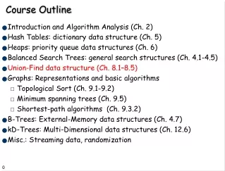
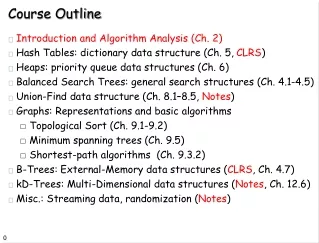
Course Outline • Introduction and Algorithm Analysis (Ch. 2) • Hash Tables: dictionary data structure (Ch. 5, CLRS) • Heaps: priority queue data structures (Ch. 6) • Balanced Search Trees: general search structures (Ch. 4.1-4.5) • Union-Find data structure (Ch. 8.1–8.5, Notes) • Graphs: Representations and basic algorithms • Topological Sort (Ch. 9.1-9.2) • Minimum spanning trees (Ch. 9.5) • Shortest-path algorithms (Ch. 9.3.2) • B-Trees: External-Memory data structures (CLRS, Ch. 4.7) • kD-Trees: Multi-Dimensional data structures (Notes, Ch. 12.6) • Misc.: Streaming data, randomization (Notes)
Introduction: 2 Motivating Applications • Imagine you are in charge of maintaining a corporate network (or a major website such as Amazon) • High speed, high traffic volume, lots of users. • Expected to perform with near perfect reliability, but is also under constant attack from malicious hackers • Monitoring what is going through the network is complex: • Why is it slow? • Which machines have become compromised? • Which applications are eating up too much bandwidth etc.
IP Network Monitoring • Any monitoring software/engine must be extremely light weight and not add to the network load • These algorithms need smart data structures to track important statistics in real time
IP Network Monitoring • Consider a simple (toy) example • Is some IP address sending a lot of data to my network? • Which IP address sent the most data in last 1 minute? • How many different IP addresses in last 5 minutes? • Have I seen this IP address in the last 5 minutes? • IP address format: 192.168.0.0 (10001011001…0010) • IPv4 has 32 bits, IPv6 has 128 bits • Cannot afford to maintain a table of all possible IP addresses to see how much traffic each is sending. • These are data structure problems, where obvious/naïve solutions are no good, and require creative/clever ideas.
Microprocessor Profiling • Modern microprocessors run at GHz or higher speeds • Yet they do an incredible amount of optimization for instruction scheduling, branch prediction etc • Profiling or monitoring code tracks performance bottlenecks, and looks for anomalies. • Compute memory access statistics • Correlations across resources etc • Toy examples: • Which memory locations used the most in the last 1 sec? • Usage map over sliding time window • Need for highly efficient dynamic data structures
A Puzzle • An abstraction: Most Frequent Item • You are shown a sequence of N positive integers • Identify the one that occurs most frequently • Example: 4, 1, 3, 3, 2, 6, 3, 9, 3, 4, 1, 12, 19, 3, 1, 9 • However, your algorithm has access to only O(1) memory • “Streaming data” • Not stored, just seen once in the order it arrives • The order of arrival is arbitrary, with no pattern • What data structure will solve this problem?
A Puzzle: Most Frequent Item • Items can be source IP addresses at a router • The most frequent IP address can be useful to monitor suspicious traffic source • More generally, find the top K frequent items • Targeted advertising • Amazon, Google, eBay, Alibaba may track items bought most frequently by various demographics
Another Puzzle • The Majority Item • You are shown a sequence of N positive integers • Identify the one that occurs at least N/2 times • A: 4, 1, 3, 3, 2, 6, 3, 9, 3, 4, 1, 12, 19, 3, 1, 9, 1 • B: 4, 1, 3, 3, 2, 3, 3, 9, 3, 4, 1, 3, 19, 3, 3, 9, 3 • Sequence A has no majority, but B has one (item 3) • Can a sequence have more than one majority? • Again, your algorithm has access to only O(1) memory • What data structure will solve this problem?
Solving the Majority Puzzle • Use two variables M (majority) and C (count). • When next item, say, X arrives • if C = 0, put M = X and C = 1; • else if M equals X, set C = C+1; • else set C = C-1; • Claim: At the end of sequence, M is the only possible candidate for majority. • Note that sequence may not have any majority. • But if there is a majority, M must be it.
Examples • Try the algorithm on following data streams: • 1, 2, 1, 1, 2, 3, 2, 2, 2, 2, 3, 2, 1 • 1, 2, 1, 2, 1, 2, 1, 2, 3, 3, 1
Proof of Correctness • Suppose item Z is the majority item. • Z must become majority candidate M at some point (why?) • While M = Z, only non-Z items cause counter to decrement • “Charge” this decrement to that non-Z item • Each non-Z item can only cancel one occurrence of Z • But in total we have fewer than N/2 non-Z items; they cannot cancel all occurrences of Z. • So, in the end, Z must be stored as M, with a non-zero count C.
Solving the Majority Puzzle • False Positives in Majority Puzzle. • What happens if the sequence does not have a majority? • M may contain a random item, with non-zero C. • Strictly, a second pass through the sequence is necessary to “confirm” that M is in fact the majority. • But in our application, it suffices to just “tag” a malicious IP address, and to monitor it for next few minutes.
Generalizing the Majority Problem • Identify k items, each appearing more than N/(k+1) times. • Note that simple majority is the case of k = 1.
Generalizing the Majority Problem • Find k items, each appearing more than N/(k+1) times. • Use k (majority, count) tuples (M1, C1), …, (Mk, Ck). • When next item, say, X arrives • if X = Mj for some j, set Cj = Cj+1 • elseif some counter i zero, set Mi = X and Ci = 1 • else decrement all counters Cj = Cj-1; • Verify for yourselves this algorithm is correct.
Back to the Most Frequent Item Puzzle • You are shown a sequence of N positive integers • Identify most frequently occurring item • Example: 4, 1, 3, 3, 2, 6, 3, 9, 3, 4, 1, 12, 19, 3, 1, 9 • Streaming model (constant amount of memory) • What clever idea will solve this problem?
An Impossibility Result • Cannot be done! • Computing the MFI requires storing Q(N) space. • An adversary based argument: • The first half of the sequence has all distinct items • At least one item, say, X is not remembered by algorithm. • In the second half, all items will be distinct, except X will occur twice, becoming the MFI.
Lessons for Data Structure Design • Puzzles such as Majority and Most Frequent Items teach us important lessons: • Elegant interplay of data structure and algorithm • To solve a problem, we should understand its structure • Correctness is intertwined with design/efficiency • Problems with superficial resemblance can have very different complexity • Do not blindly apply a data structure or algorithm without understanding the nature of the problem
130a: Design and Analysis • Foundations of Algorithm Analysis and Data Structures. • Data Structures • How to efficiently store, access, manage data • Data structures effect algorithm’s performance • Algorithm Design and Analysis: • How to predict an algorithm’s performance • How well an algorithm scales up • How to compare different algorithms for a problem
Course Objectives • Focus: systematic design and analysis of data structures (and some algorithms) • Algorithm: method for solving a problem. • Data structure: method to store information. • Guiding principles: abstraction and formal analysis • Abstraction: Formulate fundamental problem in a general form so it applies to a variety of applications • Analysis: A (mathematically) rigorous methodology to compare two objects (data structures or algorithms) • In particular, we will worry about "always correct"-ness, and worst-case bounds on time and memory (space).
Complexity and Tractability Assume the computer does 1 billion ops per sec.
Quick Review of Algorithm Analysis • Two algorithms for computing the Factorial • Which one is better? • int factorial (int n) { if (n <= 1) return 1; else return n * factorial(n-1); } • int factorial (int n) { if (n<=1) return 1; else { fact = 1; for (k=2; k<=n; k++) fact *= k; return fact; } }
A More Challenging Algorithm to Analyze main () { int x = 3; for ( ; ; ) { for (int a = 1; a <= x; a++) for (int b = 1; b <= x; b++) for (int c = 1; c <= x; c++) for (int i = 3; i <= x; i++) if(pow(a,i) + pow(b,i) == pow(c,i)) exit; x++; } }
Max Subsequence Problem • Given a sequence of integers A1, A2, …, An, find the maximum possible value of a subsequence Ai, …, Aj. • Numbers can be negative. • You want a contiguous chunk with largest sum. • Example: 4, 3, -8, 2, 6, -4, 2, 8, 6, -5, 8, -2, 7, -9, 4, -1, 5 • While not a data structure problems, it is an excellent pedagogical exercise for design, correctness proof, and runtime analysis of algorithms
Max Subsequence Problem • Given a sequence of integers A1, A2, …, An, find the maximum possible value of a subsequence Ai, …, Aj. • Example: 4, 3, -8, 2, 6, -4, 2, 8, 6, -5, 8, -2, 7, -9, 4, -1, 5 • We will discuss 4 different algorithms, of time complexity O(n3), O(n2), O(n log n), and O(n). • With n = 106, Algorithm 1 may take > 10 years; Algorithm 4 will take a fraction of a second!
Algorithm 1 for Max Subsequence Sum • Given A1,…,An , find the maximum value of Ai+Ai+1+···+Aj Return 0 if the max value is negative
Algorithm 1 for Max Subsequence Sum • Given A1,…,An , find the maximum value of Ai+Ai+1+···+Aj 0 if the max value is negative int maxSum = 0; for( int i = 0; i < a.size( ); i++ ) for( int j = i; j < a.size( ); j++ ) { int thisSum = 0; for( int k = i; k <= j; k++ ) thisSum += a[ k ]; if( thisSum > maxSum ) maxSum = thisSum; } return maxSum; • Time complexity: O(n3)
Algorithm 2 • Idea: Given sum from i to j-1, we can compute the sum from i to j in constant time. • This eliminates one nested loop, and reduces the running time to O(n2). into maxSum = 0; for( int i = 0; i < a.size( ); i++ ) int thisSum = 0; for( int j = i; j < a.size( ); j++ ) { thisSum += a[ j ]; if( thisSum > maxSum ) maxSum = thisSum; } return maxSum;
Algorithm 3 • This algorithm uses divide-and-conquer paradigm. • Suppose we split the input sequence at midpoint. • The max subsequence is • entirely in the left half, • entirely in the right half, • or it straddles the midpoint. • Example: left half | right half 4 -3 5 -2 | -1 2 6 -2 • Max in left is 6 (A1-A3); max in right is 8 (A6-A7). • But straddling max is 11 (A1-A7).
Algorithm 3 (cont.) • Example: left half | right half 4 -3 5 -2 | -1 2 6 -2 • Max subsequences in each half found by recursion. • How do we find the straddling max subsequence? • Key Observation: • Left half of the straddling sequence is the max subsequence ending with -2. • Right half is the max subsequence beginning with -1. • A linear scan lets us compute these in O(n) time.
Algorithm 3: Analysis • The divide and conquer is best analyzed through recurrence: T(1) = 1 T(n) = 2T(n/2) + O(n) • This recurrence solves to T(n) = O(n log n).
Algorithm 4 2, 3, -2, 1, -5, 4, 1, -3, 4, -1, 2
Algorithm 4 • Time complexity clearly O(n) • But why does it work? I.e. proof of correctness. 2, 3, -2, 1, -5, 4, 1, -3, 4, -1, 2 int maxSum = 0, thisSum = 0; for( int j = 0; j < a.size( ); j++ ) { thisSum += a[ j ]; if ( thisSum > maxSum ) maxSum = thisSum; else if ( thisSum < 0 ) thisSum = 0; } return maxSum; }
Proof of Correctness • Max subsequence cannot start or end at a negative Ai. • More generally, the max subsequence cannot have a prefix with a negative sum. Ex: -2 11 -4 13 -5 -2 • Thus, if we ever find that Ai through Aj sums to < 0, then we can advance i to j+1 • Proof. Suppose j is the first index after i when the sum becomes < 0 • Max subsequence cannot start at any p between i and j. Because Ai through Ap-1 is positive, so starting at i would have been even better.
Algorithm 4 int maxSum = 0, thisSum = 0; for( int j = 0; j < a.size( ); j++ ) { thisSum += a[ j ]; if ( thisSum > maxSum ) maxSum = thisSum; else if ( thisSum < 0 ) thisSum = 0; } return maxSum • The algorithm resets whenever prefix is < 0. Otherwise, it forms new sums and updates maxSum in one pass.
Why Efficient Algorithms Matter • Suppose N = 106 • A PC can read/process N records in 1 sec. • But if some algorithm does N*N computation, then it takes 1M seconds = 11 days!!! • 100 City Traveling Salesman Problem. • A supercomputer checking 100 billion tours/sec still requires 10100years! • Fast factoring algorithms can break encryption schemes. Algorithms research determines what is safe code length. (> 100 digits)
How to Measure Algorithm Performance • What metric should be used to judge algorithms? • Length of the program (lines of code) • Ease of programming (bugs, maintenance) • Memory required • Running time • Running time is the dominant standard. • Quantifiable and easy to compare • Often the critical bottleneck
Abstraction • An algorithm may run differently depending on: • the hardware platform (PC, Cray, Sun) • the programming language (C, Java, C++) • the programmer (you, me, Bill Joy) • While different in detail, all hardware and prog models are equivalent in some sense: Turing machines. • It suffices to count basic operations. • Crude but valuable measure of algorithm’s performance as a function of input size.
Average, Best, and Worst-Case • On which input instances should the algorithm’s performance be judged? • Average case: • Real world distributions difficult to predict • Best case: • Seems unrealistic • Worst case: • Gives an absolute guarantee • We will use the worst-case measure.
Asymptotic Notation Review • Big-O, “bounded above by”: T(n) = O(f(n)) • For some c and N, T(n) c·f(n) whenever n > N. • Big-Omega, “bounded below by”: T(n) = W(f(n)) • For some c>0 and N, T(n) c·f(n) whenever n > N. • Same as f(n) = O(T(n)). • Big-Theta, “bounded above and below”: T(n) = Q(f(n)) • T(n) = O(f(n)) and also T(n) = W(f(n)) • Little-o, “strictly bounded above”: T(n) = o(f(n)) • T(n)/f(n) 0 as n
By Pictures • Big-Oh (most commonly used) • bounded above • Big-Omega • bounded below • Big-Theta • exactly • Small-o • not as expensive as ...
End of Introduction and Analysis • Next Topic: Hash Tables