Plant Distribution in a Managed Land Mosaic

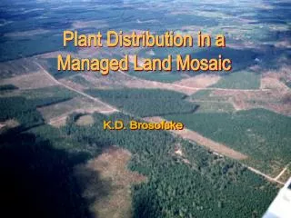
1. Plant Distribution in a Managed Land Mosaic K.D. Brosofske

2. LANDSCAPE MOSAIC Edge Matrix Patch Corridor (road)

3. Water (0.39%) Wetland (0.02%) Non-Vegetated / Recent Clearcut (4.03%) Herbs & Shrubs / Old Clearcut (18.93%) Young Hardwoods / Thickets (4.87%) Mature Hardwoods (31.31%) Jack Pine (5.44%) Red Pine (12.76%) Mixed Hardwood/Conifer (22.25%) Chequamegon N.F. Land Mosaic

4. How do landscape structure and broad-scale disturbance regime influence plant species diversity and distribution across multiple scales? • Does harvesting mimic fire in its effects on plant diversity and/or composition? • Is plant species distribution or diversity related to particular structural features or broad-scale structural patterns? • Does plant diversity vary across scales and if so, how?

5. SB: small-block clearcutting POA: thinning LB: large-block clearcutting PB: fire Broad-Scale Manipulation of Landscape Structure

6. Patch Level • Seven Patch Types (77 plots) Within Landscape • Moquah Barrens Wildlife Management Area Among Landscapes • northern Chequamegon National Forest (DFC eco-units) Multi-Scale Approach

7. Red Pine Jack Pine Young Pine Major Patch Types Clearcut Young Hardwood Hardwood Pine Barrens

8. 5 m 20 m Patch-Level Measurements • Overstory • dbh • height • age • Understory • percent cover by species • duff depth (cm) • litter (% cover and depth, cm) • coarse woody debris (CWD, % cover) • Soils • grab samples by horizon (4 pits per site) • horizons present • horizon depth • Soil Lab Analysis • pH • moisture (%) • total organic matter (%) • total N (%) • total C (%)

9. 50 40 30 20 10 2.6 2.1 1.6 1.1 0.6 a a a a a b a b a b a b a a b a Shannon Index (H’) a a Richness Y. Hardwood Pine Barrens Y. Hardwood Pine Barrens Hardwood Red Pine Jack Pine Y. Pine Clearcut Hardwood Red Pine Jack Pine Y. Pine Clearcut Plant Diversity

10. Species Composition

11. DCA Ordination of Sampling Plots DCA Axis 2 Canopy Cover (R=0.85) Soil Moisture, C-A, N-A (R=0.36-0.42) DCA Axis 1

12. Variables Used in Regression Analysis • Independent Variables • Litter cover, % • Litter depth, cm • Duff depth, cm • Coarse woody debris (CWD), % • pH of each horizon (A, E, B) • Organic matter content, % (A, E, B) • Soil moisture, % (A, E, B) • Total N content, % (A, E, B) • Total C content, % (A, E, B) • C/N ratio • Aspect/Slope Variable [ tan(slope)*cos(aspect-45), see Stage 1976 ] • Dependent Variables • Richness • Shannon Diversity Index (H’) All variables were first standardized, then transformed as needed for non-normal distributions

13. Regression Results

14. Landscape Level SB: small-block clearcuts POA: thinning LB: large-block clearcuts PB: fire

15. 5 m Transect Measurements Length: 3000+ m n=600+ plots Plot size: 1x1 m •percent cover by species •canopy cover (%) •litter cover (%) •litter depth (cm) •cwd (%) •duff depth (cm) •species, dbh, % cover overstory trees •patch type

17. 0 50 100 0 10 20 0 15 30 0 40 80 0 3 6 0 1 2 0 1000 2000 3000 MA YA1 H2 JPO SPB OPB SPB CC YA2 PA BOPB OPB H1 Select Species Distributions Pteridium aquilinum Amelanchier arborea Hieracium aurantiacum Conyza canadensis Trientalis borealis Trifolium pratense Percent Cover Distance (m) OPB

18. Transect Summary

19. Plant Species Functional Groups >1.50+ association < 0.50- association

20. Major Conclusions • Little variation existed in species diversity among patch types. • Differences in composition among patch types varied along a gradient largely related to canopy cover. • Soil & local site factors appeared important to predicting plant diversity only when broader-scale variation related to overstory structure or disturbance was reduced. PATCH LEVEL

21. Plant species responded individualistically to landscape structure. • Exotic and unique species favored roads, edges, and open/disturbed patch types disproportionately to their area in the landscape. • The pine barrens were critical to broad-scale diversity. • Harvesting did not mimic fire as a disturbance mechanism. • Effects of structural features (especially edges and roads) on plant diversity were typically clear. • Plant diversity patterns varied with resolution. LANDSCAPE LEVEL

22. Landscape structure, function, and pattern-process relationships cannot be understood properly unless an appropriate scale is used. Furthermore, examination across a range of scales is often necessary.

23. Application of Results to Predict Effects of Landscape Structure on Plants

24. Economic Products Recreation & Aesthetics Forest Management Biological Diversity Ecosystem Function & Health

25. Initial Landscape -Landsat TM -USDA FS (stand maps, OG, LTA) -USGS (roads) t = 0 Alternative Strategies Constraints -NRA -reserves -riparian zones -old-growth -etc. HARVEST model t = n t = 1 t = n t = 0 Stand Structure -basal area -height -diameter distribution -dead wood -composition t = 1 t = 0 Landscape Structure -Patches -Edges -Corridors -Matrix Stand Projection (LMS) Stand-Level Outputs Landscape-Level Outputs Plant-Habitat Relationships t = n t = n t = 1 t = 1 t = 0 t = 0 Economic Returns -cumulative value ($) Wildlife Habitat Quality -landscape composition & connectivity, interior/edge area, favored species Plant Distribution -richness & abundance -diversity index, composition Recreation -uses and users Economic Returns -saw timber, cordwood, veneer Wildlife Habitat Quality -structural diversity -favored species Plant Distribution -richness & abundance -diversity index -composition Workshop (Design & Assessment) t = t + i

26. HARVEST Simulations Using Different Strategies • total area harvested • size distribution of openings • rotation interval • spatial dispersion of harvests • constraints Current Patch Type Classification • Shrubs & Herbs • Mature Hardwoods • Young Hardwoods • Mature Red Pine • Mature Jack Pine • Young Pine • Mixed Hardwood/Pine • Wetland • New Clearcuts/Non-Vegetated • Hardwood Road Zone • Red Pine Road Zone • Pine/Clearcut Edge (in forest) • Clearcut/Pine Edge (in clearcut) • Multiple Edge Zones • Other Output (Landscape Structure) • Original Vegetation Type • Stand Age • Area • Edge Zone Occurrence • -Roads • -Different Patches

27. Current Patch Type Classification DO WE HAVE DATA FOR CURRENT PATCH TYPE? YES NO NEXT STRUCTURAL FEATURE Assign Probability and Abundance Vectors Obtained from Sampled Plots: • Species Probability In a Particular Patch Type = Sampled Frequency in 50m2 Plots • Abundance Vectors = Mean, Std. Of Sampled Abundances in 50m2 Plots

28. Generate Probability Of Occurrence By Species Does Species Occur? YES NO Generate Abundance = Probability From Normal Distribution by species With Mean and Std. Of Measured Abundance NEXT SPECIES

29. All Simulations Run for 200 Years • Buffer Patches in GIS (20 m each side) • Buffer Roads (20 m each side) • Cutting Guidelines Applied According to Distinct Management Areas • Minimum Patch Size=0.08 ha

30. Relative Area of Patch Types After Simulation Patch Type: Edge Zones Patch Interiors Percent of Total Landscape Area

31. Understory Species Richness Overall Landscape Richness = 237 species (Run 1) = 237 species (Run 5) Run 1 Run 5

32. Shannon-Wiener Diversity Index Run 1 Run 5

33. Test of the Model WT=Wetland CC=Clearcut (Herbs/Shrubs) YP=Young Pine JP=Jack Pine RP=Red Pine YH=Young Hardwoods H=Mature Hardwoods MF=Mixed Forest PRZ=Pine Road Zone HRZ=Hardwood Road Zone CEZ=Clearcut Edge Zone PEZ=Pine Edge Zone

34. Related Proposed Research (collaboration with University of Toledo)