Synchronization
Explore why synchronization is complex in distributed systems, covering mutual exclusion, concurrency, clock synchronization, and algorithms. Learn about clock mechanisms like physical and multiple clocks, synchronization methods, and logical clocks with examples like Cristian's and Berkeley algorithms. Discover the importance and implementation of clock synchronization in distributed systems.

Synchronization
E N D
Presentation Transcript
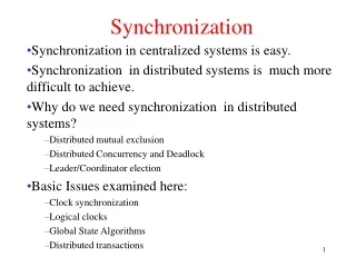
Synchronization Synchronization in centralized systems is easy. Synchronization in distributed systems is much more difficult to achieve. Why do we need synchronization in distributed systems? Distributed mutual exclusion Distributed Concurrency and Deadlock Leader/Coordinator election Basic Issues examined here: Clock synchronization Logical clocks Global State Algorithms Distributed transactions
Clock Synchronization • Example: using makefile to develop a program.. • Different machines are used for creation/compilation • When each machine has its own clock, an event that occurred after another event may nevertheless be assigned an earlier time.
Physical Clocks • Basic mechanism: Timer • A computer timer is often an oscillating quartz crystal at well defined frequencies • With the crystal there are two registers: counter, holding register. • Each oscillation of the crystal decreases the counter by one. • When the counter is ZERO • an interrupt is sent to the CPU • The counter is loaded the value of the holding counter • In this way, the crystal can create an interrupt 60 times a second. • Each such interrupt is a clock tick (and constitutes the basic timing mechanism is a centralized system).
Multiple Physical Clocks • If many CPUs are introduced time skew may develop! • Two fundamental problems need to be addressed: • How do we synchronize clocks with real-time clocks • How do we synchronize clocks with each other.
Physical Clock • Transit of the sun – solar day definition – solar second (1/864000) • The earth’s rotation is not constant! Some days are longer/shorter • than others – This lead to the introduction of the mean solar second. • TAI seconds are produced by cesium-133-atom clocks. • Computation of the mean solar day.
TAI Clocks & Leap Seconds • The introduced correction (based on TAI seconds and stays in • sync with the sun’s rotation) is • called Universal Coordinated Time (UTC) • TAI seconds are of constant length, unlike solar seconds. • Leap seconds are introduced when necessary to keep in phase with the sun.
UTC Services • Short wave radio stations broadcast a short pulse at the start of each UTC second. • MSF Station (UK) • NIST (US) • Geo-stationary Environment Operational Satellite (accurate to 0.5 msec)
Clock Synchronization Algorithms In an ideal world, Cp(t) = t where Cp(t) value clock on the machine p and t is the UTC time • The relation between clock time and UTC when clocks tick at different rates. • Maximum drift rate 1-p <= dC/dt <= 1+p • If two clocks are drifting from UTC they can be as far apart as 2p at any given time Dt.
Cristian's Clock Synch Algorithm • Requirement: if two clocks differ more than d must be • resynchronized (in software) • This must happen at least every d/2r seconds.. • Cristian’s Algorithm: send the current time from a server. • Getting the current time from a time server.
Christian’s Algorithm Problems • Two problems: • If the sender’s clock runs faster, the UTC time provided will be “earlier” – this could lead to inconsistencies (recompilation of source files etc). • Such a change should be introduced gradually • Slow down the timer of the CPU.. • How to estimate the delays for shipping messages. • (T1-T2)/2 • If you can estimate the time it takes the time server to handle the interrupt and process the incoming message I • (T1-T2-I)/2
The Berkeley Algorithm • The time daemon asks all the other machines for their clock values • The machines answer • The time daemon tells everyone how to adjust their clock
Averaging Distributed Algorithms • One class of algorithms works by dividing time into fixed-length resynchronization intervals. • The I-th interval starts at T0+ iR and runs until T0+(i+1)*R • T0 is an agreed upon moment in the past and • R is a system parameter. • At the beginning of each interval every machine broadcasts its current time. • After this broadcast, each machine starts a local timer to collect all other broadcasts with time S. • When time S elapsed the average (in each machine) is computed. • A slight variation: m lowest and n highest values (from the set collected in S period) are discarded. Why? • Examples of such protocol: NTP (Network Time Protocol).
Logical Clocks • In a network, it is important that all machines agree upon a time • This time does not need to be in sync with the time broadcasted by the radio (all the time). • In the make example, even if machines agree that it is 17:00 it does not really matter whether the UTC is 17:00:02.. • Notion of logical clock (17:00).
Logical clocks • Lamport defined the relation “happened-before” • a-> b (event a happened before event b) • The happened before relation can be observed in two settings: • If a and b are events in the same process, and a occurs before b, then a->b holds. • If a is the event of a message sent by one process, and b is the event of the message being received by another process b, then a->b holds (ie, a message cannot be received unless it has been sent)..
Logical Clocks • Happened before is transitive • If x and y happen in different processes that do not exchange messages then neither x->y nor y->x is true • The time for an event a is C(a) • If a->b then C(a) < C(b) • Logical times go always forward (corrections can be made by additions – never subtractions!)
Lamport’s Algorithm 0 0 0 8 10 6 16 20 12 24 30 18 32 24 40 40 50 30 48 36 60 56 70 42 64 80 48 72 90 54 80 100 60 60 A B C D • Three processes each with its own clock-Clocks run at different frequencies.
Lamport’s Algorithm-Solution 0 0 0 A 8 6 10 12 16 20 B 18 24 30 32 24 40 40 30 50 48 36 42 61 60 C 70 48 69 70 77 80 D 90 60 85 76 100 • Lamport’s algorithm corrects the clocks and provideds a way for total ordering of events • If a happens before b in the same process C(a)<C(b) • If a and b represent the sending and receing of a message respectively the C(a) < C(b) • For all distinctive events a and b C(a) != C(b)
Lamport Timestamps • Queries run faster when work off replicas of data • Two users (customer in San Fran and admin in NYC) • the customer from San Fran adds $100.00 to • her account (at $1000 now) • 2. the admin (from NYC) gives an increase of 1% to all accounts. • There is obviously a problem here..
Problem with Replicated Data • Problem: Updating a replicated database may leave it in an inconsistent state. • The two copies should be exactly the same!! (no matter what the order of the operations – the order does not say much about the consistency of the data; simply says that one order, or the other, should be followed). • This situation calls for a totally-orderd multicast (of operations). • How can this be done?? Can we use Lamport’s algorithm?
Sketch of the Solution • Group of processes multicasting messages to each other • Each message is always time-stamped with the time of the sender • Assume that messages from the same sender are received in the order they were sent and no messages are lost. • When a process receives a msg, put it into the local queue and the receiver multicasts a ACK to the other processes. • All processes will have the same copy (ordered) in their local queue! • Lamport’s clocks ensure that NO two messages have the same timestamps!
Global State • Global State = local states of the processes + message currently in transit. • Why knowing the Global State is useful? • If local processes have stopped and no more msgs are in transit, then we have developed a stale situation where nonone can progress (ie, something needs to be done). • Take a “distributed snapshot” • Reflects a consistent global state. • If a message has been received then it must have been sent from somewhere before! (otherwise something is wrong). • A global state can be represented by what is known as the cut. • Cuts can be consistent or inconsistent.
Cuts-Snapshots of Global State What we want to define here is an algorithm that provides an consistent Cut (snapshot) of the distributed system. • A consistent cut: one that does not include received but not sent messages! • An inconsistent cut
An Algorithm for Deriving a Distributed Snapshot • Assumptions: each process (in the DS) is connected to each other via unidirectional point-2-point comm. channels (TCP connections) • Any process may initiate the algorithm • The initiating process starts by recording its local state and then sends a MARKER along each outgoing channel (indicating that the receiver should participate in the recording of the global state).
Global State Algorithm • When a process Q receives a marker through its incoming channel C • If it has not record its own local state, it does so and sends Markers along its outgoing channels. • Otherwise, the marker that appeared on incoming channel signals that the state of the channel must be recorded (this is done by forming the sequence of messages received by Q since the last time Q recorded its state and before it received the marker). • A process has finished when it has received a marker along each of its incoming channels and processed all of them. • At that point, local state and messages in transit can be sent to a coordinator that assembles the global state.
Global State • Organization of a process and channels for a distributed snapshot
Global State • Process Q receives a marker for the first time and records its local state • Q records all incoming message • Q receives a marker for its incoming channel and finishes recording the state of the incoming channel
Distributed Computation Termination Algorithm • When a process finishes its part of the snapshot returns either a DONE or a CONTINUE message to its predecessor. • A DONE message is returned (both conds must be true) • All of Q’s successors have returned DONE messages. • Q has not received any message(s) between the point it recorded its state, and the point it had received the marker along each of its incoming channels. • In all other cases, a CONTINUE messages is sent to Q’s predecessor. • If the original initiator P receives only DONE from its successors • It means there are NO messages in transit • Therefore, computation is complete.
Election Algorithms • Many distributed applications require that one site undertakes the role of the coordinator or master • Problem: how to come up with such a master? • Each process has a unique id • Network address + id in the local space.
The Bully Algorithm The process with the higher ID (or attribute) takes over.. • 7 was the coordinator and has just crashed.. • The bully election algorithm • Process 4 holds an election • Process 5 and 6 respond, telling 4 to stop • Now 5 and 6 each hold an election
Bully Algorithm If 7 wakes-up it can hold an election and “bully” all others (takes over). • Process 6 tells 5 to stop • Process 6 wins and tells everyone
A Ring Algorithm • Assumption: processes are physically or logically ordered • Two phases: • start an ELECTION (this can be doen by more than one sites) • Once the circle is done determine the COORDINATOR (largest?) • Circulate the name of the coordinator (ie, inform everyone) • Election algorithm using a ring.
Mutual Exclusion: A Centralized Algorithm • Process 1 asks the coordinator for permission to enter a critical region. Permission is granted • Process 2 then asks permission to enter the same critical region. The coordinator does not reply. • When process 1 exits the critical region, it tells the coordinator, when then replies to 2
A Distributed Algorithm[RicartAgra81] • Two processes want to enter the same critical region at the same moment. • Process 0 has the lowest timestamp, so it wins. • When process 0 is done, it sends an OK also, so 2 can now enter the critical region.
A Toke Ring Algorithm Circulate a token – whoever has the token can get into its critical section • An unordered group of processes on a network. • A logical ring constructed in software.
Comparison • A comparison of three mutual exclusion algorithms. • The infinity indicates that the token may be aimlessly circulated in a network (if no-one wants to make use of it).
The Transaction Model • Being able to group a number of statements together in an entity that its being executed ONLY in its logical entirety. • A transaction may be concurrently executing with others in the same (or distributed) system. • Examples of transactions (xactions) • Get Euro 100.00 from your own account • Deposit Euro 25.00 in account with number 356533 • Increase all accounts by 2.7% of their balances. • The concept of transaction is supported by a few fundamental constructs.
The Transaction Model • Programming primitives for transactions.
The Transaction Model • Transaction to reserve three flights commits • Transaction aborts when third flight is unavailable
Xactions Properties • ACID- properties (or known as ACIDity). • A: atomicity • C: consistency • I : isolation • D: durability
Distributed Transactions • A nested transaction: for each one a fork is used by the parent transaction • What happens in case of failure? • A distributed transaction • Separate distributed algorithms are needed to handle management (locking) of data and commitment of the whole transaction.
Implementation of Transactions using Shadows (shadow blocks) • The file index and disk blocks for a three-block file • The situation after a transaction has modified block 0 and appended block 3 • After committing
Write Ahead Log (WAL) • If a xaction succeeds, it commits (point of no return) • Otherwise, the WAL is used to rollback to a consistent database state. • a) A transaction • b) – d) The log before each statement is executed
Concurrency Control • General organization of managers for handling transactions.
Concurrency Control • General organization of managers for handling distributed transactions.
Principle of Serializability Time (d) • a) – c) Three transactions T1, T2, and T3 • d) Possible schedules
Two-Phase Locking • Two-phase locking.
Strict Two-Phase Locking • A transaction always reads committed values • Avoids cascading aborts • Distributed 2PL: • Schedulers on each machine take care of the locks (grant/release); • Operations are forwarded to local managers.
Time Stamp Ordering • Each database item has a TSR(x) and a TSW(x) • TSR(x) is set by the xaction that most recently read the item x • TSW(x) is set by the xaction that most recently changed the value of x. • Timestamp Algorithm • Suppose that xaction Ti with TS(Ti) issues read(x) • If TS(Ti) < TSw(x) then Read needs to read a value of x that was already written by another subsequent xaction; read is rejected and Ti is rolled back. • If TS(Ti) >= TSw(x) then read is executed and TSR(x)=max{TSR(x), TS(Ti)} • Suppose that xaction Ti with TS(Ti) issues write(x) • If TS(Ti) < TSR(x) then the xaction is rejected and Ti is rolled back. • If TS(Ti) < TSw(x) then the write is rejected and Ti is rolled back. • Otherwise, the write operation is executed, and TSw(x)=TS(Ti).
Timestamp Ordering Example T1 T2 A 150 160 RT=0; WT=0 read(A) RT=150 read(A) RT=160 A:=A+1 A:=A+1 write(A) WT=160 write(A) T1 aborts!!
Timestamp Ordering • T1 T2 T3 A B C • 200 150 175 RT=0 RT=0 RT=0 • WT=0 WT=0 WT=0 • read(B) RT=200 • read(A) RT=150 • read(C) RT=175 • write(B) WT=200 • write(A) WT=200 • write(C) • ABORT T2 • write(A)